
(→Linear Time-Invariant System: Add D) |
(→Linear Time-Varying System: Add D) |
||
| Line 31: | Line 31: | ||
\begin{align} |
\begin{align} |
||
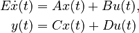
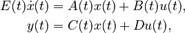
E(t)\dot{x}(t) &= A(t)x(t) + B(t)u(t),\\ |
E(t)\dot{x}(t) &= A(t)x(t) + B(t)u(t),\\ |
||
| − | y(t) &= C(t)x(t), |
+ | y(t) &= C(t)x(t) + Du(t), |
\end{align} |
\end{align} |
||
</math> |
</math> |
||
| Line 40: | Line 40: | ||
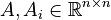
<math>A : \mathbb{R} \to \mathbb{R}^{n \times n}</math>, |
<math>A : \mathbb{R} \to \mathbb{R}^{n \times n}</math>, |
||
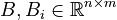
<math>B : \mathbb{R} \to \mathbb{R}^{n \times m}</math>, |
<math>B : \mathbb{R} \to \mathbb{R}^{n \times m}</math>, |
||
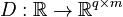
| − | <math>C : \mathbb{R} \to \mathbb{R}^{q \times n}</math> |
+ | <math>C : \mathbb{R} \to \mathbb{R}^{q \times n}</math>, |
| + | <math>D : \mathbb{R} \to \mathbb{R}^{q \times m}</math>. |
||
| − | |||
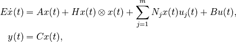
===Quadratic-Bilinear System=== |
===Quadratic-Bilinear System=== |
||
Revision as of 17:00, 8 November 2022
Benchmark Model Templates
This page specifies templates for the types of models used as benchmark systems. In particular, the naming schemes established here are used in the corresponding data sets for all benchmarks. For example,  always serves as the name of the component matrix applied to the state
  in a linear time-invariant system.
For all models we assume an input
in a linear time-invariant system.
For all models we assume an input 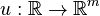 , with components
 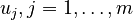 ,
a state
,
a state  ,
and an output
,
and an output  .
For all parametric models, we assume each component has
.
For all parametric models, we assume each component has  parameters; in cases where a component has fewer than parameters, the extras are treated as
  .
Some benchmarks (e.g., Bone Model) have a constant forcing term, in which case, it is assumed that
.
Some benchmarks (e.g., Bone Model) have a constant forcing term, in which case, it is assumed that  is identically
  .
.
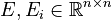
Linear Time-Invariant System
with
 ,
,
 ,
,
 ,
,
 ,
,
 .
.
Linear Time-Varying System
with
 ,
,
 ,
,
 ,
,
 ,
,
 .
.
Quadratic-Bilinear System
with
,
,
 ,
,
 ,
,
.
,
,
.
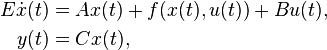
Nonlinear Time-Invariant System
with
,
,
,
,
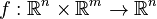 .
.
Affine Parametric Linear Time-Invariant System
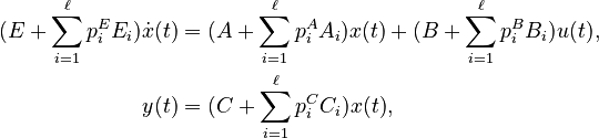
with
 ;
;
 ;
;
 ; and
; and
 ,
for all
,
for all  .
.
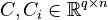
Second-Order System
with
 ,
,
,
,
 ,
,
,
,
 ,
.
,
.
When  , we denote
  .
.
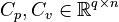
Nonlinear Second-Order System
with
,
,
,
,
 ,
,
,
.
,
,
,
.
When , we denote .
Affine Parametric Second-Order System
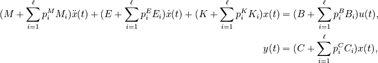
with
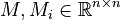 ;
;
;
;
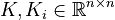 ;
; and
,
for all .
;
; and
,
for all .