Models

Benchmark Model Templates

This page specifies templates for the types of models used as benchmark systems. In particular, the naming schemes established here are used in the corresponding data sets for all benchmarks. For example, $A$ always serves as the name of the component matrix applied to the state $x(t)$ in a linear time-invariant system. For all models we assume an input $u : \mathbb{R} \to \mathbb{R}^m$, with components $u_j, j = 1, \ldots, m$, a state $x : \mathbb{R} \to \mathbb{R}^n$, and an output $y : \mathbb{R} \to \mathbb{R}^q$.

Linear Time-Invariant System

$\begin{align} E\dot{x}(t) &= Ax(t) + Bu(t),\\ y(t) &= Cx(t), \end{align}$

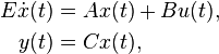
with

$E \in \mathbb{R}^{n \times n}$, $A \in \mathbb{R}^{n \times n}$, $B \in \mathbb{R}^{n \times m}$, $C \in \mathbb{R}^{q \times n}$.

Linear Time-Varying System

$\begin{align} E(t)\dot{x}(t) &= A(t)x(t) + B(t)u(t),\\ y(t) &= C(t)x(t), \end{align}$

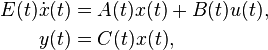
with

$E : \mathbb{R} \to \mathbb{R}^{n \times n}$, $A : \mathbb{R} \to \mathbb{R}^{n \times n}$, $B : \mathbb{R} \to \mathbb{R}^{n \times m}$, $C : \mathbb{R} \to \mathbb{R}^{q \times n}$.

Quadratic-Bilinear System

$\begin{align} E\dot{x}(t) &= A x(t) + H x(t) \otimes x(t) + \sum_{j=1}^m N_j x(t) u_j(t) + B u(t), \\ y(t) &= Cx(t), \end{align}$

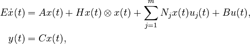
with

$E \in \mathbb{R}^{n \times n}$, $A \in \mathbb{R}^{n \times n}$, $H \in \mathbb{R}^{n \times n^2}$, $N_j \in \mathbb{R}^{n \times n}$, $B \in \mathbb{R}^{n \times m}$, $C \in \mathbb{R}^{q \times n}$.

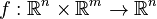
Nonlinear Time-Invariant System

$\begin{align} E\dot{x}(t) &= Ax(t) + f(x(t),u(t)) + Bu(t),\\ y(t) &= Cx(t), \end{align}$

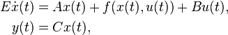
with

$E \in \mathbb{R}^{n \times n}$, $A \in \mathbb{R}^{n \times n}$, $B \in \mathbb{R}^{n \times m}$, $C \in \mathbb{R}^{q \times n}$, $f : \mathbb{R}^n \times \mathbb{R}^m \to \mathbb{R}^n$.

Affine Parametric Linear Time-Invariant System

$\begin{align} (E + \sum_{i=1}^{\ell} p^E_i E_i)\dot{x}(t) &= (A + \sum_{i=1}^{\ell} p^A_i A_i) x(t) + Bu(t),\\ y(t) &= Cx(t), \end{align}$

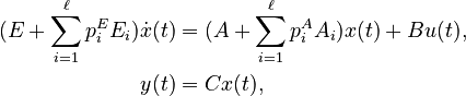
with

$E \in \mathbb{R}^{n \times n}$, $E_i \in \mathbb{R}^{n \times n}$, $A \in \mathbb{R}^{n \times n}$, $A_i \in \mathbb{R}^{n \times n}$, $B \in \mathbb{R}^{n \times m}$, $C \in \mathbb{R}^{q \times n}$.

Second-Order System

$\begin{align} M \ddot{x}(t) + E \dot{x}(t) + K x(t) &= B u(t), \\ y(t) &= C x(t), \end{align}$

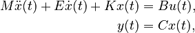
with

$M \in \mathbb{R}^{n \times n}$, $E \in \mathbb{R}^{n \times n}$, $K \in \mathbb{R}^{n \times n}$, $B \in \mathbb{R}^{n \times m}$, $C \in \mathbb{R}^{q \times n}$.

Nonlinear Second-Order System

$\begin{align} M \ddot{x}(t) + E \dot{x}(t) + K x(t) &= B u(t) + F f(x(t),u(t)), \\ y(t) &= C x(t), \end{align}$

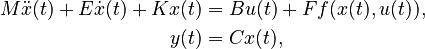
with

$M \in \mathbb{R}^{n \times n}$, $E \in \mathbb{R}^{n \times n}$, $K \in \mathbb{R}^{n \times n}$, $B \in \mathbb{R}^{n \times m}$, $F \in \mathbb{R}^{n \times n}$, $C \in \mathbb{R}^{q \times n}$, $f : \mathbb{R}^n \times \mathbb{R}^m \to \mathbb{R}^n$.

Affine Parametric Second-Order System

$\begin{align} (M + \sum_{i=1}^{\ell} p^M_i M_i)\ddot{x}(t) + (E + \sum_{i=1}^{\ell} p^E_i E_i)\dot{x}(t) + (K + \sum_{i=1}^{\ell} p^K_i K_i)x(t) &= B u(t), \\ y(t) &= C x(t), \end{align}$

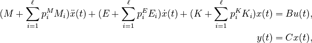
with

$M \in \mathbb{R}^{n \times n}$, $M_i \in \mathbb{R}^{n \times n}$, $E \in \mathbb{R}^{n \times n}$, $E_i \in \mathbb{R}^{n \times n}$, $K \in \mathbb{R}^{n \times n}$, $K_i \in \mathbb{R}^{n \times n}$, $B \in \mathbb{R}^{n \times m}$, $C \in \mathbb{R}^{q \times n}$.