Synthetic parametric model

Introduction

On this page you will find a synthetic parametric model for which one can easily experiment with different system orders $n$, values of the parameter $\varepsilon$, as well as different poles and residues.

Also, the decay of the Hankel singular values can be changed indirectly through the parameter $\varepsilon$.

Model description

The parameter $\varepsilon$ scales the real part of the system poles, that is, $p_i=\varepsilon a_i+jb_i$. For a system in pole-residue form

$H(s,\varepsilon) = \sum_{i=1}^{n}\frac{r_i}{s-p_i} = \sum_{i=1}^{n}\frac{r_i}{s-(\varepsilon a_i+jb_i)}$

we can write down the state-space realisation $H(s,\varepsilon) = \widehat{C}\Big(sI-\varepsilon \widehat{A}_\varepsilon - \widehat{A}_0\Big)^{-1}\widehat{B}+D$ with

$\varepsilon \widehat{A}_\varepsilon + \widehat{A}_0 = \varepsilon \left[\begin{array}{ccc} a_1 & & \\ & \ddots & \\ & & a_n\end{array}\right] +\left[\begin{array}{ccc} jb_1 & & \\ & \ddots & \\ & & jb_n\end{array}\right] ,$

$\widehat{B} = [1,\ldots,1]^T,\quad \widehat{C} = [r_1,\ldots,r_n],\quad D = 0.$

Notice that the system matrices have complex entries.

For simplicity, assume that $n$ is even, $n=2k$, and that all system poles are complex and ordered in complex conjugate pairs, i.e.

$p_1 = \varepsilon a_1+jb_1, p_2 = \varepsilon a_1-jb_1, \ldots, p_{n-1} = \varepsilon a_k+jb_k, p_n = \varepsilon a_k-jb_k,$

and the residues also form complex conjugate pairs

$r_1 = c_1+jd_1, r_2 = c_1-jd_1, \ldots, r_{n-1} = c_k+jd_k, r_n = c_k-jd_k.$

Then a realization with matrices having real entries is given by

$A_\varepsilon = \left[\begin{array}{ccc} A_{\varepsilon,1} & & \\ & \ddots & \\ & & A_{\varepsilon,k}\end{array}\right], \quad A_0 = \left[\begin{array}{ccc} A_{0,1} & & \\ & \ddots & \\ & & A_{0,k}\end{array}\right], \quad B = \left[\begin{array}{c} B_1 \\ \vdots \\ B_k\end{array}\right], \quad C = \left[\begin{array}{ccc} C_1 & \cdots & C_k\end{array}\right], \quad D = 0,$

with $A_{\varepsilon,i} = \left[\begin{array}{cc} a_i& 0 \\ 0 & a_i \end{array}\right]$, $A_{0,i} = \left[\begin{array}{cc} 0& b_i \\ -b_i & 0 \end{array}\right]$, $B_{i} = \left[\begin{array}{c} 2 \\ 0 \end{array}\right]$, $C_{i} = \left[\begin{array}{cc} c_i& d_i\end{array}\right]$.

Numerical values

We construct a system of order $n = 100$. The numerical values for the different variables are

• $a_i$ equally spaced in $[-10^3, -10]$,

• $b_i$ equally spaced in $[10, 10^3]$,

• $c_i = 1$,

• $d_i = 0$,

• $\varepsilon$$\in [1/50,1]$.

In MATLAB, the system matrices are easily formed as follows:

n = 100;
a = -linspace(1e1,1e3,n/2).';   b = linspace(1e1,1e3,n/2).';
c = ones(n/2,1);                d = zeros(n/2,1);
aa(1:2:n-1,1) = a;              aa(2:2:n,1) = a;
bb(1:2:n-1,1) = b;              bb(2:2:n-2,1) = 0;
Ae = spdiags(aa,0,n,n);
A0 = spdiags([0;bb],1,n,n) + spdiags(-bb,-1,n,n);
B = 2*sparse(mod([1:n],2)).';
C(1:2:n-1) = c.';               C(2:2:n) = d.';   C = sparse(C);

The above system matrices $A_\varepsilon, A_0, B, C$ are also available in MatrixMarket format Synth_matrices.tar.gz.

Plots

We plot the frequency response and poles for parameter values $\varepsilon \in [1/50, 1/20, 1/10, 1/5, 1/2, 1]$.

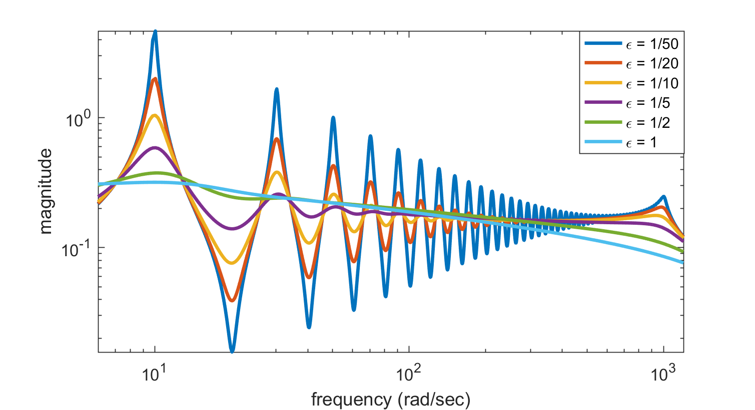
Frequency response of synthetic parametric system, for parameter values 1/50 (blue), 1/20 (green), 1/10 (red), 1/5 (teal), 1/2 (purple), 1 (yellow).

Poles of synthetic parametric system, for parameter values 1/50 (blue), 1/20 (green), 1/10 (red), 1/5 (teal), 1/2 (purple), 1 (yellow).

In MATLAB, the plots are generated using the following commands:

r(1:2:n-1,1) = c+1j*d;     r(2:2:n,1) = c-1j*d;
ep = [1/50; 1/20; 1/10; 1/5; 1/2; 1];                       % parameter epsilon
jw = 1j*linspace(0,1.2e3,5000).';                           % frequency grid
for j = 1:length(ep)
  p(:,j) = [ep(j)*a+1j*b; ep(j)*a-1j*b];                    % poles
  [jww,pp] = meshgrid(jw,p(:,j));
  Hjw(j,:) = (r.')*(1./(jww-pp));                           % freq. resp.
end
figure,  loglog(imag(jw),abs(Hjw),'LineWidth',2)
         axis tight,    xlim([6 1200])
         xlabel('frequency (rad/sec)')
         ylabel('magnitude')
         title('Frequency response for different \epsilon')
figure,  plot(real(p),imag(p),'.')
         title('Poles for different \epsilon')

Other interesting plots result for small values of the parameter. For example, for $\varepsilon = 1/100, 1/1000$, the peaks in the frequency response become more pronounced, since the poles move closer to the imaginary axis.

Next, for $\varepsilon \in [1/50, 1/20, 1/10, 1/5, 1/2, 1]$, we also plot the decay of the Hankel singular values. Notice that for small values of the parameter, the decay of the Hankel singular values is very slow.

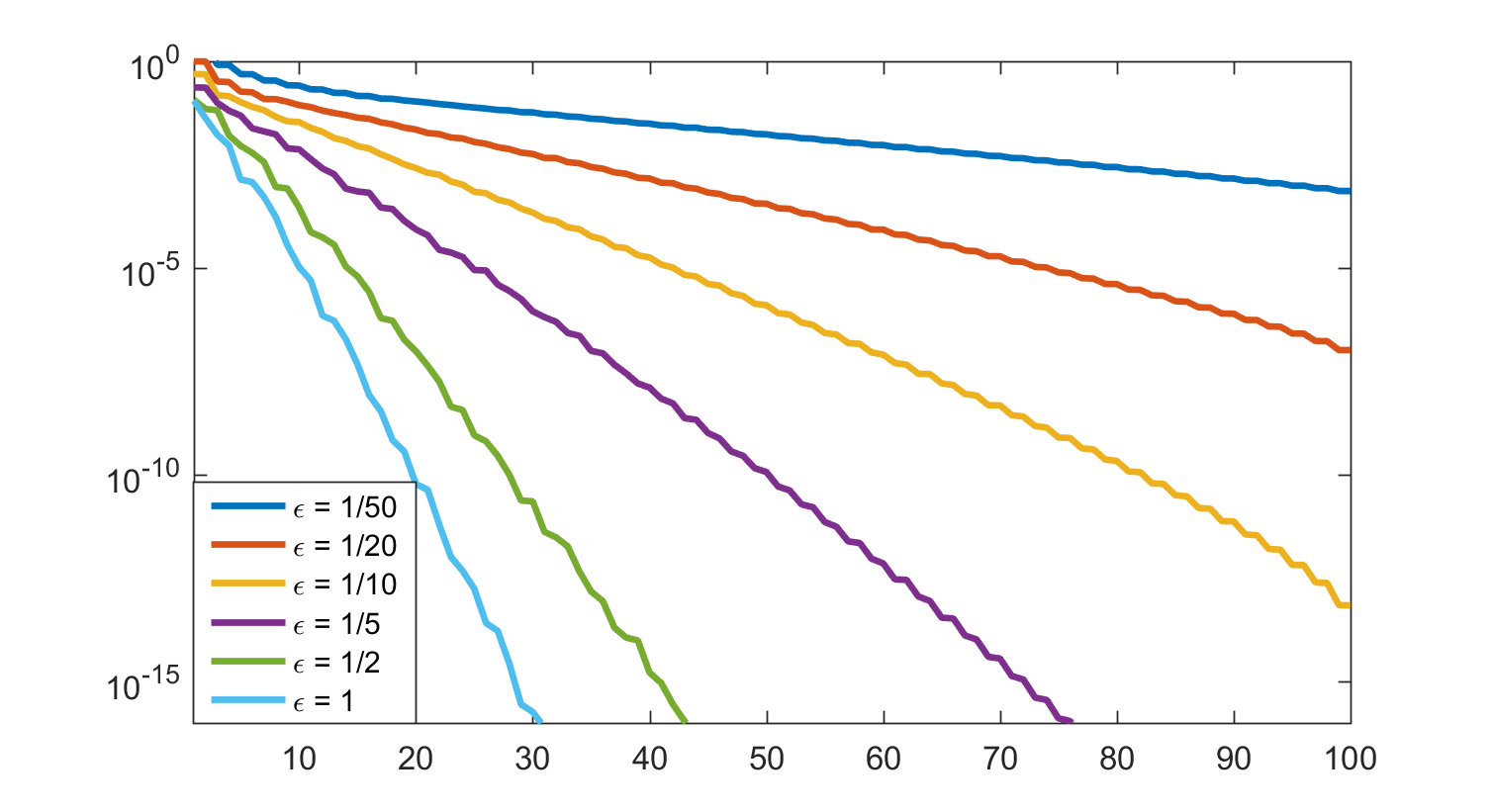
Hankel singular values of synthetic parametric system, for parameter values 1/50 (blue), 1/20 (green), 1/10 (red), 1/5 (teal), 1/2 (purple), 1 (yellow).