Branchline Coupler

Description

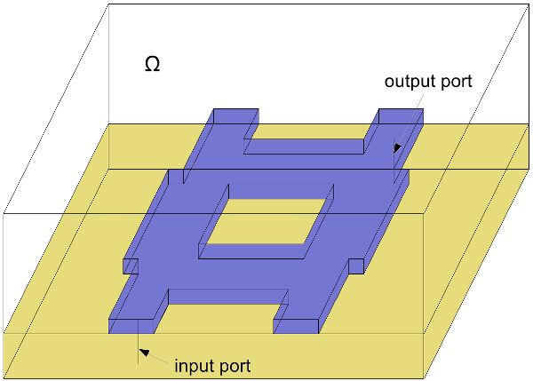
A branchline coupler is a microwave semiconductor device, which is simulated by the time-harmonic Maxwell's equation. A 2-section branchline coupler consists of four strip line ports, coupled to each other by two transversal bridges. The energy excited at one port is coupled almost in equal shares to the two opposite ports, when considered as a MIMO-system. Here, only the SISO case is considered. The branchline coupler with 0.05 mm thickness is placed on a substrate with 0.749 mm thickness and relative permittivity $\epsilon_r = 2.2$ and zero-conductivity $\sigma = 0 S/m$. The simulation domain is confined to a $23.6 \times 22 \times 7 mm^3$ box. The metallic ground plane of the device is represented by the electric boundary condition. The magnetic boundary condition is considered for the other sides of the structures. The discrete input port with source impedance 50 ohm imposes 1 A current as the input. The voltage along the coupled port at the end of the other side of the coupler is read as the output.

Matrices and Data

Considered parameters are the frequency $\omega$ and the relative permeability $\mu_r$ .

The affine form $a(u, v; \omega, \mu_r) = \sum_{q=1}^Q \Theta^q(\omega, \mu_r) a^q(u, v)$ can be established using $Q = 2$ affine terms.

The discretized bilinear form is $a(u, v; \omega, \mu_r) = \sum_{q=1}^Q \Theta^q(\omega, \mu_r) A^q$, with matrices $A^q$.

The matrices corresponding to the bilinear forms $a^q( \cdot , \cdot )$ as well as the input and output forms and the H(curl) inner product matrix have been assembled using the Finite Element Method, resulting in 27'679 degrees of freedom, after removal of boundary conditions. The files are numbered according to their appearance in the summation.

Matrices.tar.gz

The coefficient functions are given by

$\Theta^1(\omega, \mu_r) = \frac{1}{\mu_r}$

$\Theta^2(\omega, \mu_r) = -\omega^2$

The parameter domain of interest is $\omega \in [1.0, 10.0] * 10^9$ Hz, where the factor of $10^9$ has already been taken into account while assembling the matrices, while the material variation occurs between $\mu_r \in [0.5, 2.0]$. The input functional also has a factor of $\omega$.

Origin

The models have been developed within the MoreSim4Nano project.

References

[1] http://www.moresim4nano.org

[2] M. W. Hess, P. Benner, Fast Evaluation of Time-Harmonic Maxwell's Equations Using the Reduced Basis Method, MPI preprint http://www.mpi-magdeburg.mpg.de/preprints/2012/MPIMD12-17.pdf

Contact

Martin Hess