Synthetic parametric model

Introduction

On this page you will find a purely synthetic parametric model. The goal is to have a simple parametric model which one can use to experiment with different system orders, parameter values etc.

System description

The parameter $\varepsilon$ scales the real part of the system poles, that is, $p_i=\varepsilon a_i+jb_i$. For a system in pole-residue form

$H(s,\varepsilon) = \sum_{i=1}^{n}\frac{r_i}{s-p_i} = \sum_{i=1}^{n}\frac{r_i}{s-(\varepsilon a_i+jb_i)}$

we can write down the state-space realisation $H(s,\varepsilon) = \widehat{C}\Big(sI-\varepsilon \widehat{A}_\varepsilon - \widehat{A}_0\Big)^{-1}\widehat{B}+D$ with

$\varepsilon \widehat{A}_\varepsilon + \widehat{A}_0 = \varepsilon \left[\begin{array}{ccc} a_1 & & \\ & \ddots & \\ & & a_n\end{array}\right] +\left[\begin{array}{ccc} jb_1 & & \\ & \ddots & \\ & & jb_n\end{array}\right] ,$

$\widehat{B} = [1,\ldots,1]^T,\quad \widehat{C} = [r_1,\ldots,r_n],\quad D = 0.$

Notice that the system matrices have complex entries.

For simplicity, assume that $n$ is even, $n=2k$, and that all system poles are complex and ordered in complex conjugate pairs, i.e.

$p_1 = \varepsilon a_1+jb_1, p_2 = \varepsilon a_1-jb_1, \ldots, p_{n-1} = \varepsilon a_k+jb_k, p_n = \varepsilon a_k-jb_k,$

and the residues also form complex conjugate pairs

$r_1 = c_1+jd_1, r_2 = c_1-jd_1, \ldots, r_{n-1} = c_k+jd_k, r_n = c_k-jd_k.$

Then a realization with matrices having real entries is given by

$A_\varepsilon = \left[\begin{array}{ccc} A_{\varepsilon,1} & & \\ & \ddots & \\ & & A_{\varepsilon,k}\end{array}\right], \quad A_0 = \left[\begin{array}{ccc} A_{0,1} & & \\ & \ddots & \\ & & A_{0,k}\end{array}\right], \quad B = \left[\begin{array}{c} B_1 \\ \vdots \\ B_k\end{array}\right], \quad C = \left[\begin{array}{ccc} C_1 & \cdots & C_k\end{array}\right], \quad D = 0,$

with $A_{\varepsilon,i} = \left[\begin{array}{cc} a_i& 0 \\ 0 & a_i \end{array}\right]$, $A_{0,i} = \left[\begin{array}{cc} 0& b_i \\ -b_i & 0 \end{array}\right]$, $B_{i} = \left[\begin{array}{c} 2 \\ 0 \end{array}\right]$, $C_{i} = \left[\begin{array}{cc} c_i& d_i\end{array}\right]$.

Numerical values

We construct a system of order $n = 100$. The numerical values for the different variables are

• $a_i$ equally spaced in $[-10^3, -10]$,

• $b_i$ equally spaced in $[10, 10^3]$,

• $c_i = 1$,

• $d_i = 0$,

• $\varepsilon$$\in [1/50,1]$.

In MATLAB the system matrices are easily formed as follows

n = 100;
a = -linspace(1e1,1e3,n/2).';   b = linspace(1e1,1e3,n/2).';
c = ones(n/2,1);                d = zeros(n/2,1);
aa(1:2:n-1,1) = a;              aa(2:2:n,1) = a;
bb(1:2:n-1,1) = b;              bb(2:2:n-2,1) = 0;
Ae = spdiags(aa,0,n,n);
A0 = spdiags([0;bb],1,n,n) + spdiags(-bb,-1,n,n);
B = 2*sparse(mod([1:n],2)).';
C(1:2:n-1) = c.';               C(2:2:n) = d.';   C = sparse(C);

Plots

We plot the frequency response for a few different parameter values $\varepsilon \in [1/50, 1/20, 1/10, 1/5, 1/2, 1]$.

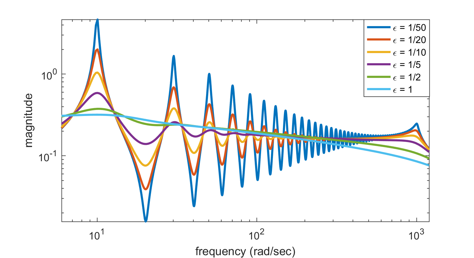
Frequency response of synthetic parametrized system, for parameter values 1/50 (blue), 1/20 (green), 1/10 (red), 1/5 (teal), 1/2 (purple), 1 (yellow).

We plot the system poles for a few different parameter values $\varepsilon \in [1/50, 1/20, 1/10, 1/5, 1/2, 1]$.

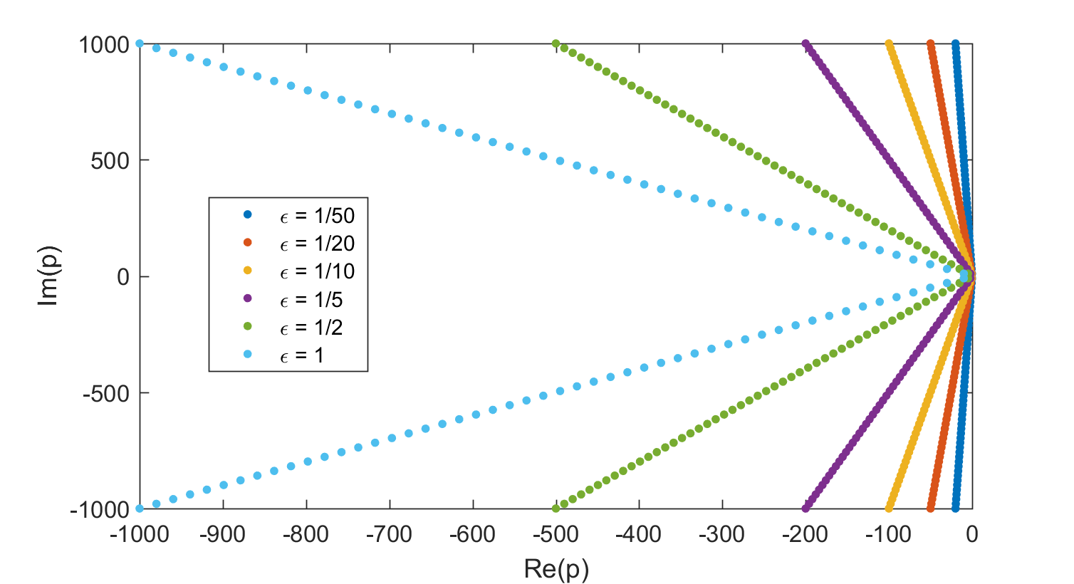
Poles of synthetic parametrized system, for parameter values 1/50 (blue), 1/20 (green), 1/10 (red), 1/5 (teal), 1/2 (purple), 1 (yellow).