| Line 20: | Line 20: | ||
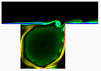
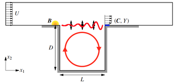
This benchmark considers a fluid-flow configuration. It consists of a two-dimensional open square cavity geometry flow problem where air flows from left to right. Such a configuration is described in details in the original work of <ref name=Barbagallo>A. Barbagallo and D. Sipp and P.J. Schmid, "Closed-loop control of an open cavity flow using reduced-order models", Journal of Fluid Mechanics, vol. 641, pp. 1-50</ref> and also (with a more dynamical system view point) in <ref name=PoussotSipp>C. Poussot-Vassal and D. Sipp, "<span class="plainlinks">[https://doi.org/10.1016/j.ifacol.2015.11.126 Parametric reduced order dynamical model construction of a fluid flow control problem]</span>", in Proceedings of the 1st IFAC Workshop on Linear Parameter Varying Systems (LPVS), Grenoble, France, 2015, pp. 133-138.</ref>, and illustrated on <xr id="fig:cavity"/> and <xr id="fig:cavityScheme"/>. | This benchmark considers a fluid-flow configuration. It consists of a two-dimensional open square cavity geometry flow problem where air flows from left to right. Such a configuration is described in details in the original work of <ref name=Barbagallo>A. Barbagallo and D. Sipp and P.J. Schmid, "Closed-loop control of an open cavity flow using reduced-order models", Journal of Fluid Mechanics, vol. 641, pp. 1-50</ref> and also (with a more dynamical system view point) in <ref name=PoussotSipp>C. Poussot-Vassal and D. Sipp, "<span class="plainlinks">[https://doi.org/10.1016/j.ifacol.2015.11.126 Parametric reduced order dynamical model construction of a fluid flow control problem]</span>", in Proceedings of the 1st IFAC Workshop on Linear Parameter Varying Systems (LPVS), Grenoble, France, 2015, pp. 133-138.</ref>, and illustrated on <xr id="fig:cavity"/> and <xr id="fig:cavityScheme"/>. | ||
For simulation purpose, the phenomena modeled by Navier and Stokes equations, is spatially discretized along a mesh composed of <math>193,874</math> triangles, corresponding to <math>n=680,974</math> degrees of freedom for the velocity variables along the <math>x</math> and <math>y</math> axis. After linearization around three fixed points for varying Reynolds numbers <math>Re=\{4000,5250,6000\}</math> three dynamical models <math>\{ | For simulation purpose, the phenomena modeled by Navier and Stokes equations, is spatially discretized along a mesh composed of <math>193,874</math> triangles, corresponding to <math>n=680,974</math> degrees of freedom for the velocity variables along the <math>x</math> and <math>y</math> axis. After linearization around three fixed points for varying Reynolds numbers <math>Re=\{4000,5250,6000\}</math> three dynamical models <math>\{H_l\}_{l=1}^3</math> can be described as a DAE realization of order <math>n=680,974</math> given as (matrices, about 100Mo each, can be provided under request to '' [[User:Poussotvassal]] '') | ||
<math> | <math> | ||
E \dot | E \dot x_l(t) = A_lx_l(t) + Bu(t) \text{ , } y(t)=Cx_l(t) \text{ where } E,A_l \in \mathbb R^{n\times n} \text{ and } B,C^T \in \mathbb R^{n} | ||
</math> | </math> | ||
| Line 36: | Line 36: | ||
Here instead, we suggest the parametric a data-driven approaches (we used the Loewner framework). We then construct the data as follows: | Here instead, we suggest the parametric a data-driven approaches (we used the Loewner framework). We then construct the data as follows: | ||
First, the frequency response <math> | First, the frequency response <math>H_l(\xi_k)</math> of each <math>l=1,\dots,3</math> configurations for frozen complex values <math>\xi_k = \xi_0 \cup \{\imath\omega_k\}_{i=k}^N</math>, with <math>\omega_i\in\mathbb R_+</math>, <math>\xi_0\in\mathbb R</math> and <math>k=1,\dots,100</math> is computed. | ||
Second, ten intermediate parametric configurations between each <math>j</math>-th Reynolds numbers configuration are constructed by linear interpolation of the frequency responses <math> | Second, ten intermediate parametric configurations between each <math>j</math>-th Reynolds numbers configuration are constructed by linear interpolation of the frequency responses <math>H_l(\xi_k)</math>, leading to <math>\{\rho_l\}_{l=1}^M\in\mathbb R</math>, for <math>l=1,\dots,M=31</math> configurations. | ||
===Considered data=== | ===Considered data=== | ||
| Line 46: | Line 46: | ||
<math> | <math> | ||
\{\ | \{\xi_k,\rho_l,H_{kl}\}_{k=1,l=1}^{N+1,M}, | ||
</math> | </math> | ||
where <math>H_{ | where <math>H_{kl}\in\mathbb C</math> represents the transfer from the input signal (upward cavity pressure) to the measurement output (downward cavity pressure), evaluated at varying complex values <math>\xi_k = 0.1 \cup \{\imath\omega_k\}_{k=1}^N</math> and parameters <math>\{\rho_l\}_{l=1}^M\in\mathbb R</math>, for <math>j=1,\dots,M=31</math>. Specifically, the frequencies are between xxHz until yyHz in steps of zzHz, and parameters are from 1 to 3 in steps of zz. | ||
==Origin== | ==Origin== | ||
Revision as of 08:39, 9 June 2021
 Note: This page has not been verified by our editors.
Description
Motivation
This benchmark considers a fluid-flow configuration. It consists of a two-dimensional open square cavity geometry flow problem where air flows from left to right. Such a configuration is described in details in the original work of [1] and also (with a more dynamical system view point) in [2], and illustrated on xx--CrossReference--dft--fig:cavity--xx and xx--CrossReference--dft--fig:cavityScheme--xx.
For simulation purpose, the phenomena modeled by Navier and Stokes equations, is spatially discretized along a mesh composed of triangles, corresponding to degrees of freedom for the velocity variables along the and axis. After linearization around three fixed points for varying Reynolds numbers three dynamical models can be described as a DAE realization of order given as (matrices, about 100Mo each, can be provided under request to User:Poussotvassal )
where the input is the vertical pressure actuator located upstream of the cavity and the output is a shear stress sensor, located downstream of the cavity. In this particular case, the parameter is the Reynolds number . The transfer functions read
In [2], the IRKA approach (being a realization based -oriented reduction method) is used to sequentially approximate each realization with a low dimensional one. Then, the interpolation along the parameter is done in a second step by interpolating each coefficients in the canonical basis of the obtained realization.
Here instead, we suggest the parametric a data-driven approaches (we used the Loewner framework). We then construct the data as follows:
First, the frequency response of each configurations for frozen complex values , with , and is computed. Second, ten intermediate parametric configurations between each -th Reynolds numbers configuration are constructed by linear interpolation of the frequency responses , leading to , for configurations.
Considered data
The proposed benchmark contains a set of complex-domain responses provided at varying real parametric values. The numerical values are inspired (but slightly modified) from the reference paper given below and are given as Matlab file. More specifically, the data provided in this use-case are given as the triple:
where represents the transfer from the input signal (upward cavity pressure) to the measurement output (downward cavity pressure), evaluated at varying complex values and parameters , for . Specifically, the frequencies are between xxHz until yyHz in steps of zzHz, and parameters are from 1 to 3 in steps of zz.
Origin
Collaboration between ONERA DTIS (dynamical systems and information departement) and DAAA (Fluid mechanics departement). The data come from a fluid simulator (coded in FreeFem++). The model is constructed by D. Sipp and post-processing was performed jointly by P. Vuillemin and C. Poussot-Vassal.
Data
Description
The FlexibleAircraft.zip (aaMB) repository contains three files:
- The dataONERA_OpenCavity.mat data file, with
- p : the parametric values (real vector).
- s0 : the evaluation of the parametric transfer function at a frozen real (real vector).
- w : the frequency values in rad/s (real vector).
- H : transfer function matrix evaluation at different frequeny points and parametric values (complex matrix).
- The dataONERA_OpenCavity_withMOR.mat data file, with 3 ROMs obtained with the MOR toolbox using the parametric Loewner method
- Hr1 : linear parametric rational ROMs with varying dimensions (state-space models in Matlab form).
- The startONERA_OpenCavityt.m script file, used to loads and plots the data for illustration.
Objective
Find a linear (stable?) parametric reduced order model that well approximates the data. Note that stability property is very promising.
Citation
To cite this benchmark, use the following references:
- For the benchmark itself and its data:
- The MORwiki Community, Fluid Flow Linearized Open Cavity Model. MORwiki - Model Order Reduction Wiki, 2021. https://morwiki.mpi-magdeburg.mpg.de/morwiki/index.php/Fluid_Flow_Linearized_Open_Cavity_Model
- For the background on the benchmark with a dynamical and control engineering point of view:
@inproceedings{PoussotLPVS:2015,
  author    = {C. Poussot-Vassal and  D. Sipp},
  title     = {Parametric reduced order dynamical model construction of a fluid flow control problem},
  booktitle = {Proceedings of the 1st IFAC Workshop on Linear Parameter Varying Systems},
  address   = {Grenoble, France},
  month     = {October},
  year      = {2015},
  pages     = {133-138},
}
- For the background on the benchmark with a fluid-flow point of view:
@article{Barbagallo:2008,
  author  = {A. Barbagallo and D. Sipp and P.J. Schmid},
  journal = {Journal of Fluid Mechanics},
  pages   = {1-50},
  title   = {Closed-loop control of an open cavity flow using reduced-order models},
  volume  = {641},
  year    = {2008}
}
References
- ↑ A. Barbagallo and D. Sipp and P.J. Schmid, "Closed-loop control of an open cavity flow using reduced-order models", Journal of Fluid Mechanics, vol. 641, pp. 1-50
- ↑ 2.0 2.1 C. Poussot-Vassal and D. Sipp, "Parametric reduced order dynamical model construction of a fluid flow control problem", in Proceedings of the 1st IFAC Workshop on Linear Parameter Varying Systems (LPVS), Grenoble, France, 2015, pp. 133-138.

