Thermal Block

Thermal Block

Background
Benchmark ID	thermalBlock_n7488m1q4
Category	misc
System-Class	AP-LTI-FOS
Parameters
nstates	7488
ninputs	1
noutputs	4
nparameters	4
components	A, B, C, E
Copyright
License	BSD 2-Clause "Simplified" License
Creator	Jens Saak
Editor	Jens Saak Christian Himpe Petar Mlinarić
Location
https://zenodo.org/record/3691894/files/ABCE.mat

Description

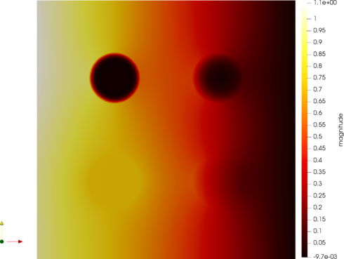
A parametric semi-discretized heat transfer problem with varying heat transfer coefficients, the parameters, on subdomains. This model is also called the cookie baking problem, and can be viewed as a flattened 2-D version of the skyscraper problem from high-performance computing.

Figure 1: The computational domain and boundaries.

Figure 2: A sample heat distribution at time 1.0 for parameter choice [100, 0.01, 0.001, 0.0001].

Figure 3: Sigma magnitude plot of the single parameter variant.

Modeling

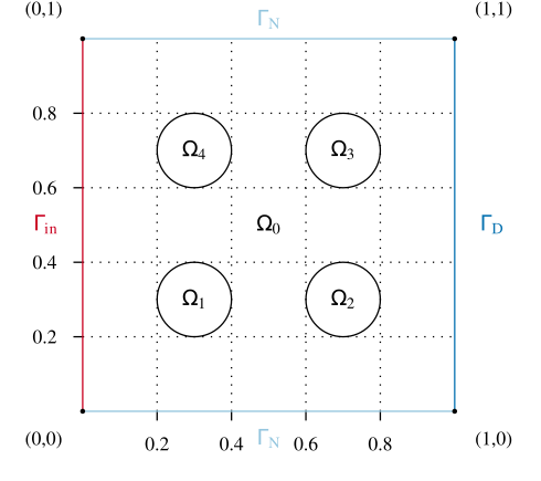
Consider a parameter $\mu\in{[10^{-6},10^2]}^4\subset\mathbb{R}^{4}$ and define the heat conductivity $\sigma(\xi; \mu)$ as $1.0$ when $\xi\in\Omega_0$ and $\sigma(\xi; \mu)=\mu_i$ when $\xi\in\Omega_i$. The heat distribution is governed by the equation:

$\partial_t \theta(t, \xi; \mu) + \nabla \cdot (- \sigma(\xi; \mu) \nabla \theta(t, \xi; \mu)) = 0,\text{ for } t\in (0,T), \text{ and } \xi \in \Omega,$

with a heat-inflow condition on the left (Neumann boundary)

$\sigma(\xi; \mu) \nabla \theta(t, \xi; \mu) \cdot n(\xi) = u(t)\text{ for } t \in (0,T), \text{ and } \xi \in \Gamma_{in},$

perfect isolation on the top and bottom (Neumann-zero boundary)

$\sigma(\xi; \mu) \nabla \theta(t, \xi; \mu) \cdot n(\xi) = 0\text{ for } t \in (0,T), \text{ and } \xi \in \Gamma_N,$

and fixed temperature on the right (Dirichlet boundary)

$\theta(t, \xi; \mu) = 0\text{ for } t \in (0,T), \text{ and } \xi \in \Gamma_{D},$

and initial condition

$\theta(0, \xi; \mu) = 0 \text{ for } \xi \in \Omega.$

Discretization

For the discretization, FEniCS 2019.1 was used on a simplicial grid with first order elements. The mesh is generated from the domain specification using gmsh 3.0.6 with 'clscale' set to $0.1$. The Python-based source code for the discretization can be found at Zenodo.

Origin

This benchmark was developed for the MODRED 2019 proceedings.

Data

The benchmark includes the basic domain description as a gmsh input file, Python scripts for the matrix assembly, simulation in pyMOR, and visualization as VTK, together with the matrices both as one combined file ABCE.mat or separate matrix market files for all matrices. The sources and the ABCE.mat are available for download at Zenodo.

Note that the heat transfer coefficients are designed as characteristic functions on the domains, such that the system is only well-posed when all entries in $\mu$ are positive.

Dimensions

System structure:

$\begin{align} E\dot{x}(t) &= (A_1 + \mu_1 A_2 + \mu_2 A_3 + \mu_3 A_4 + \mu_4 A_5) x(t) + Bu(t), \\ y(t) &= Cx(t) \end{align}$

System dimensions:

$E \in \mathbb{R}^{N \times N}$, $A_{1,...,5} \in \mathbb{R}^{N \times N}$, $B \in \mathbb{R}^{N \times 1}$, $C \in \mathbb{R}^{4 \times N}$,

where $N=7\,488$ for the system matrices given in ABCE.mat.

Variants

Besides the full four parameter setup, the model can be used in variations with other numbers of independent parameters. The following two are recommended in the original work and have been investigated in the literature,,,.

Single parameter

The interpretation of the thermal block as the "cookie baking" problem with slight variation in the dough leads to an easy one parameter variant. Here the new single parameter $\hat\mu\in [ 10^{-6}, 10^2]$ is chosen such that $\mu = \hat\mu\left[0.2, 0.4, 0.6, 0.8\right].$

Non-parametric

The system can be used as a standard LTI state-space model. It is suggested to use $\mu = \sqrt{10} [0.2, 0.4, 0.6, 0.8]$.

Citation

To cite this benchmark, use the following references:

• For the benchmark itself and its data:

S. Rave and J. Saak, Thermal Block. MORwiki - Model Order Reduction Wiki, 2020. https://modelreduction.org/morwiki/Thermal_Block

@MISC{morwiki_thermalblock,
  author =       {Rave, S. and Saak, J.},
  title =        {Thermal Block},
  howpublished = {{MORwiki} -- Model Order Reduction Wiki},
  url =          {https://modelreduction.org/morwiki/Thermal_Block},
  year =         2020
}

• For the background on the benchmark:

S. Rave and J. Saak, A Non-Stationary Thermal-Block Benchmark Model for Parametric Model Order Reduction. e-prints 2003.00846, arXiv, math.NA (2020).

@INPROCEEDINGS{morRavS21,
  author =       {Rave, S. and Saak, J.},
  title =        {A Non-Stationary Thermal-Block Benchmark Model for Parametric Model Order Reduction},
  booktitle =    {Model Reduction of Complex Dynamical Systems},
  series =       {International Series of Numerical Mathematics},
  volume =       {171},
  publisher =    {Springer},
  year =         2021,
  doi =          {10.1007/978-3-030-72983-7_16}
}

Contact

Jens Saak

References

- ↑ S. Rave, J. Saak, An Non-Stationary Thermal-Block Benchmark Model for Parametric Model Order Reduction, Model Reduction of Complex Dynamical Systems, International Series of Numerical Mathematics 171: 349-356, 2021.
- ↑ P. Benner, S. W. R. Werner, MORLAB -- the Model Order Reduction LABoratory, Model Reduction of Complex Dynamical Systems, International Series of Numerical Mathematics 171: 393--415, 2021.
- ↑ C. Himpe, Comparing (empirical-Gramian-based) model order reduction algorithms, Model Reduction of Complex Dynamical Systems, International Series of Numerical Mathematics 171: 141--164, 2021.
- ↑ P. Benner, M. Köhler, J. Saak, Matrix equations, sparse solvers: M-M.E.S.S.-2.0.1 – philosophy, features and application for (parametric) model order reduction, Model Reduction of Complex Dynamical Systems, International Series of Numerical Mathematics 171: 369--392, 2021.
- ↑ P. Mlinarić, S. Rave, J. Saak, Parametric model order reduction using pyMOR, Model Reduction of Complex Dynamical Systems, International Series of Numerical Mathematics 171: 357--367 , 2021.