Difference between revisions of "Batch Chromatography"

Revision as of 13:58, 21 November 2012

Description of physical model

Preparative liquid chromatography as a crucial separation and purification tool has been widely employed in food, fine chemical and pharmaceutical industries. Chromatographic separation at industry scale can be operated either discontinuously or in a continuous mode. The continuous case will be addressed in the benchmark SMB, and here we focus on the discontinuous mode -- batch chromatography.

The dynamics of the batch chromatographics column can be described precisely by an axially dispersed plug-flow model with a limited mass-transfer rate characterized by a linear driving force (LDF) approximation. In this model the differential mass balance of component $i$ ( $i=A,B,$ ) in the liquid phase can be written as:

$\frac{\partial c_i}{\partial t}+\frac{1-\epsilon}{\epsilon}\frac{\partial q_i}{\partial t}+u\frac{\partial c_i}{\partial z}-D_i\frac{\partial^2 c_i}{\partial z^2}=0, \qquad z\in(0,\;L), \qquad [1]$

where $c_i$ and $q_i$ are the concentrations of solute $i$ in the liquid and solid phases, respectively, $u$ the interstitial liquid velocity, $\epsilon$ the column porosity, $t$ the time coordinate, $z$ the axial coordinate along the column, $L$ the column length, $D_i=uL/Pe$ the axial dispersion coefficient and $Pe$ the P\'{e}clet number. The adsorption rate is modeled by the LDF approximation:

$\frac{\partial q_i}{\partial t} = K_{m,i}\,(q^{Eq}_i-q_i), \qquad z\in[0,\;L], \qquad [2]$

where $K_{m,i}$ is the mass-transfer coefficient of component $i$ and $q^{Eq}_i$ is the adsorption equilibrium concentration calculated by the isotherm equation for component $i$ . Here the bi-Langmuir isotherm model is used to describe the adsorption equilibrium:

$q^{Eq}_i=\frac{H_{i,1}\,c_i}{1+\sum_{j=A,B}K_{j,1}\,c_j}+\frac{H_{i,2}\,c_i}{1+\sum_{j=A,B}K_{j,2}\,c_j},\; i=A,B, \qquad [3]$ where $H_{i,1}$ and $H_{i,2}$ are the Henry constants, and $K_{j,1}$ and $K_{j,2}$ the thermodynamic coefficients.

The boundary conditions for Eq. [] are specified by the Danckwerts relations:

$D_i\left.\frac{\partial c_i}{\partial z}\right|_{z=0} = u\,(\left.c_i\right|_{z=0}-c^{in}_i), \quad\quad \left.\frac{\partial c_i}{\partial z}\right|_{z=L}=0, \qquad [4]$

where $c^{in}_i$ is the concentration of component $i$ at the inlet of the column. A rectangular injection is assumed for the system and thus

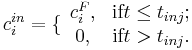
$c^{in}_i=\{ \begin{array}{cc} c^F_i, &\text{if} t \le t_{inj};\\ 0, &\text{if} t > t_{inj}. \end{array}$

where $c^F_i$ is the feed concentration for component $i$ and $t_{inj}$ is the injection period. In addition, the column is assumed unloaded initially:

$c_i(t=0,z)=q_i(t=0,z)=0,\quad z\in[0,\;L],\;i=A,B. \qquad [5]$

Discretization

@@ Line 14: / Line 14: @@
 <math>
-\frac{\partial c_i}{\partial t}+\frac{1-\epsilon}{\epsilon}\frac{\partial q_i}{\partial t}+u\frac{\partial c_i}{\partial z}-D_i\frac{\partial^2 c_i}{\partial z^2}=0, \qquad z\in(0,\;L),
+\frac{\partial c_i}{\partial t}+\frac{1-\epsilon}{\epsilon}\frac{\partial q_i}{\partial t}+u\frac{\partial c_i}{\partial z}-D_i\frac{\partial^2 c_i}{\partial z^2}=0, \qquad z\in(0,\;L), \qquad [1]
 </math>
 where <math>c_i</math> and <math>q_i</math> are the concentrations of solute $i$ in the liquid and solid phases, respectively, $u$ the interstitial liquid velocity, <math>\epsilon</math> the column porosity, <math>t</math> the time coordinate, <math>z</math> the axial coordinate along the column, <math>L</math> the column length, <math>D_i=uL/Pe</math> the axial dispersion coefficient and <math>Pe</math> the P\'{e}clet number. The adsorption rate is modeled by the LDF approximation:
 <math>
-\frac{\partial q_i}{\partial t} = K_{m,i}\,(q^{Eq}_i-q_i), \qquad z\in[0,\;L],
+\frac{\partial q_i}{\partial t} = K_{m,i}\,(q^{Eq}_i-q_i), \qquad z\in[0,\;L], \qquad [2]
 </math>
 where <math>K_{m,i}</math> is the mass-transfer coefficient of component <math>i</math> and <math>q^{Eq}_i</math> is the adsorption equilibrium concentration calculated by the isotherm equation for component <math>i</math>. Here the bi-Langmuir isotherm model is used to describe the adsorption equilibrium:
 <math>
-q^{Eq}_i=\frac{H_{i,1}\,c_i}{1+\sum_{j=A,B}K_{j,1}\,c_j}+\frac{H_{i,2}\,c_i}{1+\sum_{j=A,B}K_{j,2}\,c_j},\; i=A,B,
+q^{Eq}_i=\frac{H_{i,1}\,c_i}{1+\sum_{j=A,B}K_{j,1}\,c_j}+\frac{H_{i,2}\,c_i}{1+\sum_{j=A,B}K_{j,2}\,c_j},\; i=A,B,  \qquad [3]
 </math>
 where <math>H_{i,1}</math> and <math>H_{i,2}</math> are the Henry constants, and <math>K_{j,1}</math> and <math>K_{j,2}</math> the thermodynamic coefficients.
@@ Line 31: / Line 33: @@
 <math>
-D_i\left.\frac{\partial c_i}{\partial z}\right|_{z=0} = u\,(\left.c_i\right|_{z=0}-c^{in}_i), \quad\quad \left.\frac{\partial c_i}{\partial z}\right|_{z=L}=0,
+D_i\left.\frac{\partial c_i}{\partial z}\right|_{z=0} = u\,(\left.c_i\right|_{z=0}-c^{in}_i), \quad\quad \left.\frac{\partial c_i}{\partial z}\right|_{z=L}=0,  \qquad [4]
 </math>
@@ Line 37: / Line 39: @@
 <math>
+c^{in}_i=\{ \begin{array}{cc}  c^F_i,  &\text{if} t \le t_{inj};\\
-c^{in}_i=
+,  &\text{if} t >   t_{inj}.
-\begin{cases}
+\end{array}
-  c^F_i,  &\text{if $t \le t_{inj}$;}\\
-,  &\text{if $t >   t_{inj}$.}
-\end{cases}
 </math>
 where <math>c^F_i</math> is the feed concentration for component <math>i</math> and <math>t_{inj}</math> is the injection period. In addition, the column is assumed unloaded initially:
 <math>
-c_i(t=0,z)=q_i(t=0,z)=0,\quad z\in[0,\;L],\;i=A,B.
+c_i(t=0,z)=q_i(t=0,z)=0,\quad z\in[0,\;L],\;i=A,B.  \qquad [5]
 </math>