
| Line 72: | Line 72: | ||
The data of the system matrices <math>E, D_1, D_2, A, B, C</math> as well as the initial state <math>\vec{c}_0=x_0</math> are in MatrixMarket format. The interesting output of the model is the current which is computed by <math>I(t)=C(5,:)\vec{c}</math> in MATLAB notation. The interested plot of the output is called the cyclic voltammogram, which is the plot of the current changing with the voltage <math>u(t)</math>. |
The data of the system matrices <math>E, D_1, D_2, A, B, C</math> as well as the initial state <math>\vec{c}_0=x_0</math> are in MatrixMarket format. The interesting output of the model is the current which is computed by <math>I(t)=C(5,:)\vec{c}</math> in MATLAB notation. The interested plot of the output is called the cyclic voltammogram, which is the plot of the current changing with the voltage <math>u(t)</math>. |
||
| − | Fig.1 [[File: |
+ | Fig.1 [[File: Fig.1.jpg]] |
Revision as of 17:00, 18 November 2011
Description of the process
Scanning Electrochemical Microscopy (SECM) finds many applications in current problems in the biological field. Quantitative mathematical models have been developed for different operating modes of the SECM. Except for some very specific problems, like the diffusion-controlled current on a circular electrode far away from the border, solutions can only be obtained by numerical simulation, which is based on discretization of the model in space by an appropriate method like finite differences, finite elements, or boundary elements. After discretization, a high-dimensional system of ordinary differential equations is obtained. Its high dimensionality leads to high computational cost.
We consider a cylindrical electrode in Fig.1. The computation domain under the 2D-axisymmetrical approximation includes the electrolyte under the electrode. We assume that the concentration does not depend on the rotation angle. A single chemical reaction takes place on the electrode:
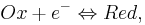 (1)
(1)
where  and
and  are two different species in the reaction.
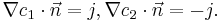
According to the theory of SECM [2], the species transport in the electrolyte is described by diffusion only. The diffusion partial differential equation is given by the second Fick law as follows
are two different species in the reaction.
According to the theory of SECM [2], the species transport in the electrolyte is described by diffusion only. The diffusion partial differential equation is given by the second Fick law as follows
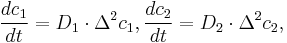
where  and
and  is the concentration field of species and respectively. The initial conditions are
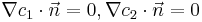
 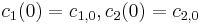 . Conditions at the glass and the bottom of the bath are described by the Neumann boundary conditions of zero flux
 . Conditions at the border to the bulk are described by Dirichlet boundary conditions of constant concentration, equal to the initial conditions
  ,
,  . The boundary conditions at the electrode are described by
Here  is related to the forward reaction rate
  and the backward reaction rate
  through the Buttler-Volmer equation,
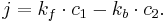
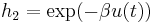
The reaction rate $k_f$ and $k_b$ are in the follow forms,

Here,  is the heterogeneous standard rate constant, and is an empirical transmission factor for a heterogeneous reaction.
  is the Faraday-constant,
  is the gas constant,
  is the temperature and
  is the number of exchanged electrons per reaction.
 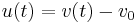 is the difference between the electrode potential and the reference potential. This difference, to which we refer below as voltage, is changed during the measurement of a voltammogram.
Description of the model
The control volume method has been used for the spatial discretization of(1). Together with the boundary conditions, the resulted system of ordinary differential equations are as follows,
where E and  are system matrices, is a function of voltage that in turn depends on time. The voltage appears in the system matrix due to the boundary conditions~(\ref{b3}). The vector
  is the vector of unknown concentrations, which includes both the Ox and Red species. The vector
  is the load vector, which arises as a consequence of the Dirichlet boundary conditions imposed at the bulk boundary of the electrolyte. The total current is computed as an integral (sum) over the electrode surface.
The matrix has the following form,
is the load vector, which arises as a consequence of the Dirichlet boundary conditions imposed at the bulk boundary of the electrolyte. The total current is computed as an integral (sum) over the electrode surface.
The matrix has the following form,

where 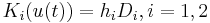 , and
, and 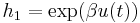 ,
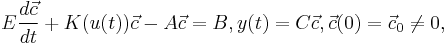
,  with . The the voltage
  is a function of
  ,
,
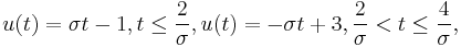
where can take four different values,  . The constant
  is computed from the parameters
  , and , giving a value of
  .
.
Although the system is a time-varying system, it can be considered as a parametrized systems with two parameters  and
and  .
.
Data information
The data of the system matrices  as well as the initial state
  are in MatrixMarket format. The interesting output of the model is the current which is computed by
  in MATLAB notation. The interested plot of the output is called the cyclic voltammogram, which is the plot of the current changing with the voltage .
Fig.1 File:Fig.1.jpg