Reduced Basis PMOR method

The Reduced Basis Method (RBM) we present here is applicable to static and time-dependent linear PDEs.

Time-Independent PDEs

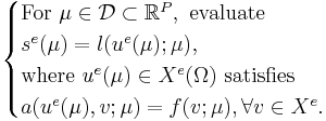
The typical model problem of the RBM consists of a parametrized PDE stated in weak form with bilinear form $a(\cdot, \cdot; \mu)$ and linear form $f(\cdot; \mu)$. The parameter $\mu$ is considered within a domain $\mathcal{D}$ and we are interested in an output quantity $s(\mu)$ which can be expressed via a linear functional of the field variable $l(\cdot; \mu)$.

The exact, infinite-dimensional formulation, indicated by the superscript e, is given by

$\begin{cases} \text{For } \mu \in \mathcal{D} \subset \mathbb{R}^P, \text{ evaluate } \\ s^e(\mu) = l(u^e(\mu);\mu), \\ \text{where } u^e(\mu) \in X^e(\Omega) \text{ satisfies } \\ a(u^e(\mu),v;\mu) = f(v;\mu), \forall v \in X^e. \end{cases}$

We assume a large-scale discretization to be given, such that we consider

$\begin{cases} \text{For } \mu \in \mathcal{D} \subset \mathbb{R}^P, \text{ evaluate } \\ s(\mu) = l(u(\mu);\mu), \\ \text{where } u(\mu) \in X(\Omega) \text{ satisfies } \\ a(u(\mu),v;\mu) = f(v;\mu), \forall v \in X. \end{cases}$

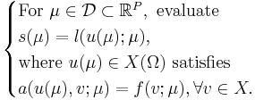
The underlying assumption of the RBM is that the parametrically induced manifold 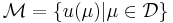$\mathcal{M} = \{u(\mu) | \mu \in \mathcal{D}\}$ can be approximated by a low dimensional space $V_N$.

It also applies the concept of an offline-online decomposition, in that a large pre-processing offline cost is acceptable in view of a very low online cost (of a reduced order model) for each input-output evaluation, when in a many-query or real-time context.

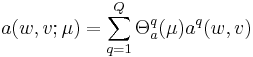
The essential assumption which allows the offline-online decomposition is that there exists an affine parameter dependence

$a(w,v;\mu) = \sum_{q=1}^Q \Theta_a^q(\mu) a^q(w,v)$

$f(v;\mu) = \sum_{q=1}^{Q^f} \Theta_f^{q}(\mu) f^q(v).$

The Lagrange Reduced Basis space is established by iteratively choosing Lagrange parameter samples

$S_N = \{\mu^1,...,\mu^N\}$

and considering the associated Lagrange RB spaces 

$V_N = \text{span}\{u^\mathcal{N}(\mu^n), 1 \leq n \leq N \}$

in a greedy sampling.

This leads to hierarchical RB spaces: 

$V_1 \subset V_2 \subset ... \subset V_{N_{max}}$.