
| Line 23: | Line 23: | ||
\end{cases} |
\end{cases} |
||
</math> |
</math> |
||
| + | |||
| + | We assume a large-scale discretization to be given, such that we consider |
||
| + | |||
| + | <math> |
||
| + | \begin{cases} |
||
| + | \text{For } \mu \in \mathcal{D} \subset \mathbb{R}^P, \text{ evaluate } \\ |
||
| + | s(\mu) = l(u(\mu);\mu), \\ |
||
| + | \text{where } u(\mu) \in X(\Omega) \text{ satisfies } \\ |
||
| + | a(u(\mu),v;\mu) = f(v;\mu), \forall v \in X. |
||
| + | \end{cases} |
||
| + | </math> |
||
| + | |||
| + | The underlying assumption of the RBM is that the parametrically induced manifold <math> \mathcal{M} = \{u(\mu) | \mu \in \mathcal{D}\} </math> |
||
| + | can be approximated by a low dimensional space <math> V_N </math>. |
||
| + | |||
| + | It also applies the concept of an offline-online decomposition, in that a large pre-processing offline cost is acceptable in view |
||
| + | of a very low online cost (of a reduced order model) for each input-output evaluation, when in a many-query or real-time context. |
||
| + | |||
| + | |||
| + | |||
==Time-Dependent PDEs== |
==Time-Dependent PDEs== |
||
Revision as of 15:16, 19 November 2012
The Reduced Basis Method (RBM) we present here is applicable to static and time-dependent linear PDEs.
Time-Independent PDEs
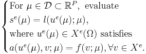
The typical model problem of the RBM consists of a parametrized PDE stated in weak form with
bilinear form  and linear form
  .
The parameter
.
The parameter  is considered within a domain
  and we are interested in an output quantity
  which can be
expressed via a linear functional of the field variable
which can be
expressed via a linear functional of the field variable  .
.
The exact, infinite-dimensional formulation, indicated by the superscript e, is given by
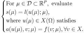
We assume a large-scale discretization to be given, such that we consider
The underlying assumption of the RBM is that the parametrically induced manifold 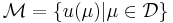 can be approximated by a low dimensional space
  .
.
It also applies the concept of an offline-online decomposition, in that a large pre-processing offline cost is acceptable in view of a very low online cost (of a reduced order model) for each input-output evaluation, when in a many-query or real-time context.