
| (199 intermediate revisions by 9 users not shown) | |||
| Line 1: | Line 1: | ||
[[Category:benchmark]] |
[[Category:benchmark]] |
||
| + | [[Category:Parametric]] |
||
| + | [[Category:Sparse]] |
||
| + | [[Category:linear]] |
||
| + | [[Category:time varying]] |
||
| + | [[Category:first differential order]] |
||
| + | [[Category:ODE]] |
||
| + | [[Category:MIMO]] |
||
| + | [[Category:CRC-TR-96]] |
||
| + | {{Infobox |
||
| + | |Title = Vertical Stand |
||
| + | |Benchmark ID = |
||
| + | * verticalStandParametric_n16626m6q27 |
||
| + | * verticalStandSwitched_n16626m6q27 |
||
| + | |Category = misc |
||
| + | |System-Class = AP-LTV-FOS |
||
| + | |nstates = 16626 |
||
| + | |ninputs = 6 |
||
| + | |noutputs = 27 |
||
| + | |nparameters = |
||
| + | * 234 |
||
| + | * 11 |
||
| + | |components = A, B, C, E |
||
| + | |License = NA |
||
| + | |Creator = [[User:Lnor]] |
||
| + | |Editor = |
||
| + | * [[User:Lnor]] |
||
| + | * [[User:Saak]] |
||
| + | * [[User:Himpe]] |
||
| + | |Zenodo-link = NA |
||
| + | }} |
||
| + | |||
| + | __NUMBEREDHEADINGS__ |
||
==Description== |
==Description== |
||
| + | <figure id="fig:cad"> |
||
| − | The vertical stand represents a structural part of a machine tool. On one of its surfaces there are guide rails located. On these rails a tool slide is moving due to the machining process the slide has to perform by the machine tool on top. The machining process producing a certain amount of heat which is transported through the structure into the vertical stand. This heat source will be considered as an temperature input at the guide rails. This transfered heat amount will lead to deformations within the device induced by the prevailed temperature field. The evolution of this field is modeled by the heat equation |
||
| + | [[File:Staender_Geom_white.jpg|180px|thumb|right|<caption>CAD Geometry</caption>]] |
||
| + | </figure> |
||
| + | The '''vertical stand''' (see Fig. 1) represents a structural part of a machine tool. A pair of guide rails is located on one of the surfaces of this structural part, |
||
| − | <math> |
||
| + | and during the machining process, a tool slide is moved to different positions along these rails. The machining process produces a certain amount of heat which is transported through the slide structure into the '''vertical stand'''. This heat source is considered to be a temperature input <math>q_{th}(t)</math> at the guide rails. The induced temperature field, denoted by <math> T </math> is modeled by the [[wikipedia:heat equation|heat equation]] |
||
| + | |||
| + | :<math> |
||
| + | c_p\rho\frac{\partial{T}}{\partial{t}}-\Delta T=0 |
||
| + | </math> |
||
| + | |||
| + | with the boundary conditions |
||
| + | |||
| + | :<math> |
||
| + | \lambda\frac{\partial T}{\partial n}=q_{th}(t) \qquad\qquad\qquad |
||
| + | </math> on <math> \Gamma_{rail} </math> (surface where the tool slide is moving on the guide rails), |
||
| + | |||
| + | describing the heat transfer between the tool slide and the '''vertical stand'''. |
||
| + | The heat transfer to the ambiance is given by the locally fixed [[wikipedia:Robin_boundary_condition|Robin-type boundary condition]] |
||
| + | |||
| + | :<math> |
||
| + | \lambda\frac{\partial T}{\partial n}=\kappa_i(T-T_i^{ext}) |
||
| + | </math> on <math> \Gamma_{amb} </math> (remaining boundaries). |
||
| + | |||
| + | The motion driven temperature input and the associated change in the temperature field <math>T</math> lead to deformations <math>u</math> within the stand structure. Further, it is assumed that no external forces <math>q_{el}</math> are induced to the system, such that the deformation is purely driven by the change of temperature. Since the mechanical behavior of the machine stand is much faster than the propagation of the thermal field, it is sufficient to consider the stationary [[wikipedia:Linear_elasticity|linear elasticity]] equations |
||
| + | :<math> |
||
\begin{align} |
\begin{align} |
||
| + | -\operatorname{div}(\sigma(u)) &=q_{el}=0&\text{ on }\Omega,\\ |
||
| − | c_p\rho\frac{\partial{x}}{\partial{t}}=\nabla.(\lambda\nabla x)&=0\qquad in \Omega\times(0,T)\\ |
||
| + | \varepsilon(u) &= {\mathbf{C}}^{-1}:\sigma(u)+\beta(T-T_{ref})I_d&\text{ on }\Omega,\\ |
||
| − | \lambda\partial_\nu x&=q \qquad on \Gamma_s |
||
| + | {\mathbf{C}}^{-1}\sigma(u) &=\frac{1+\nu}{E_u}\sigma(u)-\frac{\nu}{E_u}\text{tr}(\sigma(u))I_d&\text{ on }\Omega,\\ |
||
| + | \varepsilon(u) &= \frac{1}{2}(\nabla u+\nabla u^T)&\text{on }\Omega. |
||
\end{align} |
\end{align} |
||
</math> |
</math> |
||
| + | '''Geometrical dimensions:''' |
||
| − | Contact information: |
||
| + | |||
| + | Stand: Width (<math>x</math> direction): <math>519mm</math>, Height (<math>y</math> direction): <math>2\,010mm</math>, Depth (<math>z</math> direction): <math>480mm</math> |
||
| + | |||
| + | Guide rails: <math>y\in [519, 2\,004] mm</math> |
||
| + | |||
| + | Slide: Width: <math>430 mm</math>, Height: <math>500mm</math>, Depth: <math>490 mm</math> |
||
| + | |||
| + | |||
| + | ===Discretized Model=== |
||
| + | The solid model has been generated and meshed in [[wikipedia:ANSYS|ANSYS]]. |
||
| + | For the spatial discretization the [[wikipedia:finite element method|finite element method]] with linear Lagrange elements has been used and is implemented in [[wikipedia:FEniCS Project|FEniCS]]. The resulting system of [[wikipedia:ordinary differential equations|ordinary differential equations (ODE)]], representing the thermal behavior of the stand, reads |
||
| + | |||
| + | :<math> |
||
| + | \begin{align} |
||
| + | E \frac{\partial}{\partial t} T(t) &= A(t)T(t) + B(t)z(t), \\ |
||
| + | T(0) &= T_0, |
||
| + | \end{align} |
||
| + | </math> |
||
| + | |||
| + | with <math>t>0</math> and a system dimension of <math>n=16\,626</math> degrees of freedom and <math>m=6</math> inputs. Note that <math>A(.)\in\mathbb{R}^{n\times n}</math> and <math>B(.)\in\mathbb{R}^{n\times m}</math> are time-dependent matrix-valued functions. That is, the underlying model is represented by a linear time-Varying (LTV) state-space system. More precisely, here the time dependence originates from the change of the boundary condition on <math>\Gamma_{rail}</math> due to the motion of the tool slide. The system input is, according to the boundary conditions, given by |
||
| + | :<math> |
||
| + | z_i=\begin{cases} |
||
| + | q_{th}(t), i=1,\\ |
||
| + | \kappa_i T_i^{ext}(t), i=2,\dots,6 |
||
| + | \end{cases}. |
||
| + | </math> |
||
| + | <!-- |
||
| + | The heat load <math>f</math> induced by the slide and the external temperatures <math>T_i^{ext}</math> serve as the inputs <math> z_i </math> of the corresponding state-space system. |
||
| + | --> |
||
| + | The discretized stationary elasticity model becomes |
||
| + | :<math> |
||
| + | Mu(t)=KT(t). |
||
| + | </math> |
||
| + | For the observation of the displacements in single points/regions of interest an output equation of the form |
||
| + | :<math> |
||
| + | y(t) = C u(t) |
||
| + | </math> |
||
| + | is given. |
||
| + | |||
| + | Exploiting the one-sided coupling of the temperature and deformation fields, and reorganizing the elasticity equation in the form <math>u(t)=M^{-1}KT(t)</math>, the heat equation and the elasticity model can easily be combined via the output equation. Finally, the thermo-elastic control system is of the form |
||
| + | :<math> |
||
| + | \begin{align} |
||
| + | E \frac{\partial}{\partial t} T(t) &= A(t)T(t) + B(t)z(t), \\ |
||
| + | y(t)& = \tilde{C}T(t),\\ |
||
| + | T(0) &= T_0, |
||
| + | \end{align} |
||
| + | </math> |
||
| + | where the modified output matrix <math>\tilde{C}=CM^{-1}KT(t)</math> includes the entire elasticity information. |
||
| + | |||
| + | The motion of the tool slide and the associated variation of the affected input boundary are modeled by two different system representations. The following specific model representations have been developed and investigated in <ref name="morLanSB14" />, <ref name="LanSB15" />, <ref name="Lan17" />. |
||
| + | |||
| + | ===Switched Linear System=== |
||
| + | <figure id="fig:segm"> |
||
| + | [[File:Slide_stand_scheme_new.pdf|thumb|right|220px|<caption>Schematic segmentation</caption>]] |
||
| + | </figure> |
||
| + | |||
| + | For the model description as a switched linear system, the guide rails of the machine stand are modeled as fifteen equally distributed horizontal segments with a height of <math>99mm</math> (see a schematic depiction in Fig. 2). Any of these segments is assumed to be completely covered by the tool slide if its midpoint (in y-direction) lies within the height of the slide. On the other hand, each segment whose midpoint is not covered is treated as not in contact and therefore the slide always covers five to six segments at each time. Still, the covering of six segments does not have a significant effect on the behavior of the temperature and displacement fields. Due to that and in order to keep the number of subsystems small, this scenario will be neglected. Then, in fact eleven distinct, discrete boundary condition configurations for the stand model that are prescribed by the geometrical dimensions of the segmentation and the tool slide are defined. These distinguishable setups define the subsystems |
||
| + | :<math> |
||
| + | \begin{align} |
||
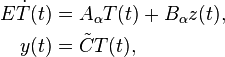
| + | E\dot{T}(t)&=A_{\alpha}T(t)+B_{\alpha}z(t),\\ |
||
| + | y(t)&=\tilde{C}T(t), |
||
| + | \end{align} |
||
| + | </math> |
||
| + | of the switched linear system <ref name=Lib03/>, where <math>\alpha</math> is a piecewise constant function of time, which takes its value from the index set <math>\mathcal{J}=\{1,\dots,11\}</math>. To be more precise, the switching signal <math>\alpha</math> implicitly maps the slide position to the number of the currently active subsystem. |
||
| + | |||
| + | ===Linear Parameter-Varying System=== |
||
| + | For the parametric model description, the finite element nodes located at the guide rails are clustered with respect to their y-coordinates. This results in <math>233</math> distinct layers in y-direction. According to these layers, the matrices <math>A(t)=A(\mu(t)), B(t)=B(\mu(t)) </math> are defined in a parameter-affine representation of the form |
||
| + | :<math> |
||
| + | \begin{align} |
||
| + | A(\mu) = A_0+f_1(\mu)A_1+...+f_{m_A}(\mu)A_{m_A},\\ |
||
| + | B(\mu) = B_0+g_1(\mu)B_1+...+g_{m_B}(\mu)B_{m_B} |
||
| + | \end{align} |
||
| + | </math> |
||
| + | with the scalar functions <math>f_i,g_j\in\{0,1\}, i=1,...,m_A, j=1,...,m_B</math> selecting the active layers, covered by the tool slide and <math>\mu(t)</math> being the position of the middle point (vertical / y-direction) of the slide. The matrix <math>A_0\in\mathbb{R}^{n\times n}</math> consists of the discretization of the [[wikipedia:Laplace operator|Laplacian]] <math>\Delta</math>, as well as the discrete portions from the Robin-type boundaries that correspond to the temperature exchange with the ambiance. The remaining summands <math>A_j\in\mathbb{R}^{n\times n},~j=1,...,m_A</math> denote the discretization associated to the moving Robin-type boundaries. For the representation of the input matrix, the summand <math>B_0\in\mathbb{R}^{n\times 6}</math> consists of a single zero column followed by five columns related to the inputs <math>z_i,~i=2,...,6</math>. The remaing matrices <math>B_j,~j=1,...,m_B</math> are built by a single column corresponding to the different layers followed by a zero block of dimension <math>n\times 5</math> designated to fit the dimension of <math>B_0</math>. |
||
| + | |||
| + | Note that in general, the number of summands of these representations need not be equal. Still, according to the number of layers, for this example, it holds that <math>m_A=m_B=233</math>. For more details on parametric models, see e.g., <ref name="morBauBBetal11" /> and the references therein. |
||
| + | |||
| + | Then, the final linear parameter-varying (LPV) reformulation of the above LTV system reads |
||
| + | :<math> |
||
| + | \begin{align} |
||
| + | E\dot{T}(t)&=A(\mu)T(t)+B(\mu)z(t),\\ |
||
| + | y(t)&=\tilde{C}T(t). |
||
| + | \end{align} |
||
| + | </math> |
||
| + | |||
| + | ==Acknowledgement & Origin== |
||
| + | The base model was developed <ref name="GalGM11" />, <ref name="GalGM15" /> in the [http://transregio96.de Collaborative Research Centre Transregio 96] ''Thermo-Energetic Design of Machine Tools'' funded by the [http://www.dfg.de/en/index.jsp Deutsche Forschungsgemeinschaft] . |
||
| + | |||
| + | ==Data== |
||
| + | ====Switched System Data==== |
||
| + | The data file [[Media:VertStand_SLS.tar.gz|VertStand_SLS.tar.gz]] contains the matrices |
||
| + | <!-- |
||
| + | {| class="wikitable" style="margin: auto; text-align:right;" |
||
| + | |+ style="caption-side:bottom;"| |
||
| + | |- |
||
| + | |mtx-File |
||
| + | |matrix |
||
| + | |dimension |
||
| + | |- |
||
| + | |E.mtx |
||
| + | |<math>E</math> |
||
| + | |<math>n\times n</math> |
||
| + | |- |
||
| + | |A<math>\alpha</math>.mtx |
||
| + | |<math>A_\alpha, \alpha=1,\dots,11</math> |
||
| + | |<math>n\times n</math> |
||
| + | |- |
||
| + | |B<math>\alpha</math>.mtx |
||
| + | |<math>B_\alpha, \alpha=1,\dots,11</math> |
||
| + | |<math>n\times m</math> |
||
| + | |- |
||
| + | |C.mtx |
||
| + | |<math>\tilde{C}</math> |
||
| + | |<math>q\times n</math> |
||
| + | |} |
||
| + | --> |
||
| + | |||
| + | :<math> |
||
| + | \begin{align} |
||
| + | E\in\mathbb{R}^{n\times n}, \tilde{C}\in\mathbb{R}^{q\times n}, A_\alpha\in\mathbb{R}^{n\times n}, B_\alpha\in\mathbb{R}^{n\times m}, \alpha=1,\dots,11. |
||
| + | \end{align} |
||
| + | </math> |
||
| + | defining the subsystems of the switched linear system. |
||
| + | The matrices <math>A_\alpha</math> and <math>B_\alpha</math> are numbered according to the slide position in descending order (1 - uppermost slide position / 11 - lowest slide position). |
||
| + | |||
| + | System dimensions: |
||
| + | :<math> |
||
| + | n=16\,626, m=6, q=27 |
||
| + | </math> |
||
| + | |||
| + | ====Parametric System Data==== |
||
| + | The data file [[Media:VertStand_PAR.tar.gz|VertStand_PAR.tar.gz]] contains the matrices |
||
| + | |||
| + | :<math> |
||
| + | E,A_j\in\mathbb{R}^{n\times n},j=1,...,234, B_{rail}\in\mathbb{R}^{n\times 233}, B_{amb}\in\mathbb{R}^{n\times 5}</math> and <math>\tilde{C}\in\mathbb{R}^{q\times n}, q=27, n=16\,626, |
||
| + | </math> |
||
| + | as well as a file ''ycoord_layers.mtx'' containing the y-coordinates of the layers located on the guide rails. |
||
| + | |||
| + | Here <math>B_{rail} </math> contains all columns corresponding to the different layers on the guide rails and <math>B_{amb}</math> correlates to the boundaries where the ambient temperatures act on. |
||
| + | |||
| + | In order to set up the parameter dependent matrices <math>A(\mu),B(\mu)</math> the active matrices <math>A_i</math> and columns <math>B_{rail}(:,i)</math> associated to the covered layers have to be identified by the current position <math>\mu(t)</math> (vertical middle point of the slide) and the geometrical dimensions of the tool slide and the y-coordinates of the different layers given in ''ycoord_layers.mtx''. Then, <math>B(\mu)</math> has to be set up in the form <math>B(\mu)=[\sum_{i\in id_{active}}\!\!\!\!\!B_{rail}(:,i),B_{amb}]</math>, where <math>id_{active}</math> denotes the set of covered layers and their corresponding columns in <math>B_{rail}</math>. |
||
| + | |||
| + | |||
| + | <!-- |
||
| + | The matrix . |
||
| + | The first column is responsible for the input of the temperature at the clamped bottom slice of the structure. |
||
| + | Column 2 describes the ... part of the stand. Columns 3 to 5 describe different thresholds with respect to the height of ambient air temperature. |
||
| + | The third column includes the nodes of the lower third <math>(y\in[0,670)mm)</math> of the stand. |
||
| + | In column 4 all nodes of the middle third <math>(y\in[670,1\,340)mm)</math> of the geometry are contained |
||
| + | and the fifth column of <math>B_{surf}</math> includes the missing upper <math>(y\in[1\,340,2\,010]mm)</math> part. |
||
| + | --> |
||
| + | |||
| + | The matrices have been re-indexed (starting with 1) for [[MORB]]. |
||
| + | |||
| + | ==Citation== |
||
| + | |||
| + | To cite this benchmark, use the following references: |
||
| + | |||
| + | * For the benchmark itself and its data: |
||
| + | ::The MORwiki Community, '''Vertical Stand'''. MORwiki - Model Order Reduction Wiki, 2018. https://modelreduction.org/morwiki/Vertical_Stand |
||
| + | |||
| + | @MISC{morwiki_vertstand, |
||
| + | author = <nowiki>{{The MORwiki Community}}</nowiki>, |
||
| + | title = {Vertical Stand}, |
||
| + | howpublished = {{MORwiki} -- Model Order Reduction Wiki}, |
||
| + | url = <nowiki>{https://modelreduction.org/morwiki/Vertical_Stand}</nowiki>, |
||
| + | year = 2014 |
||
| + | } |
||
| + | |||
| + | * For the background on the benchmark: |
||
| + | |||
| + | @Article{morLanSB14, |
||
| + | author = {Lang, N. and Saak, J. and Benner, P.}, |
||
| + | title = {Model Order Reduction for Systems with Moving Loads}, |
||
| + | journal = {at-Automatisierungstechnik}, |
||
| + | volume = 62, |
||
| + | number = 7, |
||
| + | pages = {512--522}, |
||
| + | year = 2014, |
||
| + | doi = {10.1515/auto-2014-1095} |
||
| + | } |
||
| + | |||
| + | ==References== |
||
| + | |||
| + | <references> |
||
| + | |||
| + | <ref name="morBauBBetal11"> U. Baur, C. A. Beattie, P. Benner, and S. Gugercin, |
||
| + | "<span class="plainlinks">[http://epubs.siam.org/doi/abs/10.1137/090776925 Interpolatory projection methods for parameterized model reduction]</span>", |
||
| + | SIAM J. Sci. Comput., 33(5):2489-2518, 2011</ref> |
||
| + | |||
| + | <ref name="Lib03">D. Liberzon, <span class="plainlinks">[https://doi.org/10.1007/978-3-319-12625-8_8 Switching in Systems and Control] </span>, Springer-Verlag, New York, 2003</ref> |
||
| + | |||
| + | <ref name="GalGM11"> A. Galant, K. Großmann, and A. Mühl, Model Order Reduction (MOR) for |
||
| + | Thermo-Elastic Models of Frame Structural Components on Machine Tools. |
||
| + | ANSYS Conference & 29th CADFEM Users’ Meeting 2011, October |
||
| + | 19-21, 2011, Stuttgart, Germany</ref>. |
||
| + | |||
| + | <ref name="morLanSB14">N. Lang and J. Saak and P. Benner, |
||
| + | <span class="plainlinks">[https://doi.org/10.1515/auto-2014-1095 Model Order Reduction for Systems with Moving Loads] </span>, |
||
| + | in De Gruyter Oldenbourg: at-Automatisierungstechnik, Volume 62, Issue 7, Pages 512-522, 2014</ref> |
||
| + | |||
| + | <ref name="LanSB15">N. Lang, J. Saak and P. Benner, <span class="plainlinks">[https://doi.org/10.1007/978-3-319-12625-8_8 Model Order Reduction for Thermo-Elastic Assembly Group Models] </span>, In: Thermo Energetic Design of Machine Tools, Lecture Notes in Production Engineering, 85-92, 2015</ref> |
||
| + | |||
| + | <ref name="Lan17">N. Lang, <span class="plainlinks">[https://www.logos-verlag.de/cgi-bin/buch/isbn/4700 Numerical Methods for Large-Scale Linear Time-Varying Control Systems and related Differential Matrix Equations] </span>, Logos-Verlag, 2018. ISBN: 978-3-8325-4700-4</ref> |
||
| + | |||
| + | <ref name="GalGM15">A. Galant, K. Großmann and A. Mühl, <span class="plainlinks">[https://doi.org/10.1007/978-3-319-12625-8_7 Thermo-Elastic Simulation of Entire Machine Tool] </span>, In: Thermo Energetic Design of Machine Tools, Lecture Notes in Production Engineering, 69-84, 2015</ref> |
||
| + | |||
| + | </references> |
||
| + | |||
| + | ==Contact== |
||
| − | '' [[User: |
+ | '' [[User:Saak]]'' |
Latest revision as of 06:42, 17 June 2025
| Background | |
|---|---|
| Benchmark ID |
|
| Category |
misc |
| System-Class |
AP-LTV-FOS |
| Parameters | |
| nstates |
16626
|
| ninputs |
6 |
| noutputs |
27 |
| nparameters |
|
| components |
A, B, C, E |
| Copyright | |
| License |
NA |
| Creator | |
| Editor | |
| Location | |
|
NA | |
1 Description

The vertical stand (see Fig. 1) represents a structural part of a machine tool. A pair of guide rails is located on one of the surfaces of this structural part,
and during the machining process, a tool slide is moved to different positions along these rails. The machining process produces a certain amount of heat which is transported through the slide structure into the vertical stand. This heat source is considered to be a temperature input  at the guide rails. The induced temperature field, denoted by
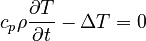
  is modeled by the heat equation
with the boundary conditions
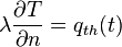 on
on  (surface where the tool slide is moving on the guide rails),
describing the heat transfer between the tool slide and the vertical stand. The heat transfer to the ambiance is given by the locally fixed Robin-type boundary condition
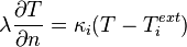 on
on  (remaining boundaries).
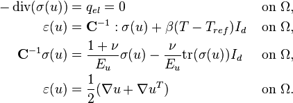
The motion driven temperature input and the associated change in the temperature field lead to deformations  within the stand structure. Further, it is assumed that no external forces
  are induced to the system, such that the deformation is purely driven by the change of temperature. Since the mechanical behavior of the machine stand is much faster than the propagation of the thermal field, it is sufficient to consider the stationary linear elasticity equations
Geometrical dimensions:
Stand: Width ( direction):
  , Height (
 direction):
  , Depth (
 direction):
Guide rails: ![y\in [519, 2\,004] mm](/morwiki/images/math/d/6/6/d6623742beb91c8320ac3a3a6356fe02.png)
Slide: Width:  , Height:
  , Depth:
1.1 Discretized Model
The solid model has been generated and meshed in ANSYS. For the spatial discretization the finite element method with linear Lagrange elements has been used and is implemented in FEniCS. The resulting system of ordinary differential equations (ODE), representing the thermal behavior of the stand, reads
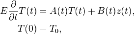
with  and a system dimension of
  degrees of freedom and
  inputs. Note that
 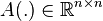 and
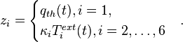
and 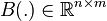 are time-dependent matrix-valued functions. That is, the underlying model is represented by a linear time-Varying (LTV) state-space system. More precisely, here the time dependence originates from the change of the boundary condition on due to the motion of the tool slide. The system input is, according to the boundary conditions, given by
The discretized stationary elasticity model becomes

For the observation of the displacements in single points/regions of interest an output equation of the form
is given.
Exploiting the one-sided coupling of the temperature and deformation fields, and reorganizing the elasticity equation in the form  , the heat equation and the elasticity model can easily be combined via the output equation. Finally, the thermo-elastic control system is of the form
where the modified output matrix  includes the entire elasticity information.
The motion of the tool slide and the associated variation of the affected input boundary are modeled by two different system representations. The following specific model representations have been developed and investigated in [1], [2], [3].
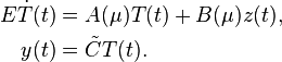
1.2 Switched Linear System
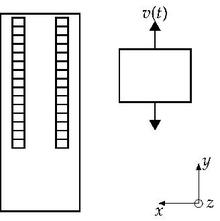
For the model description as a switched linear system, the guide rails of the machine stand are modeled as fifteen equally distributed horizontal segments with a height of  (see a schematic depiction in Fig. 2). Any of these segments is assumed to be completely covered by the tool slide if its midpoint (in y-direction) lies within the height of the slide. On the other hand, each segment whose midpoint is not covered is treated as not in contact and therefore the slide always covers five to six segments at each time. Still, the covering of six segments does not have a significant effect on the behavior of the temperature and displacement fields. Due to that and in order to keep the number of subsystems small, this scenario will be neglected. Then, in fact eleven distinct, discrete boundary condition configurations for the stand model that are prescribed by the geometrical dimensions of the segmentation and the tool slide are defined. These distinguishable setups define the subsystems
of the switched linear system [4], where  is a piecewise constant function of time, which takes its value from the index set
  . To be more precise, the switching signal implicitly maps the slide position to the number of the currently active subsystem.
1.3 Linear Parameter-Varying System
For the parametric model description, the finite element nodes located at the guide rails are clustered with respect to their y-coordinates. This results in  distinct layers in y-direction. According to these layers, the matrices
  are defined in a parameter-affine representation of the form

with the scalar functions  selecting the active layers, covered by the tool slide and
  being the position of the middle point (vertical / y-direction) of the slide. The matrix
  consists of the discretization of the Laplacian
  , as well as the discrete portions from the Robin-type boundaries that correspond to the temperature exchange with the ambiance. The remaining summands
  denote the discretization associated to the moving Robin-type boundaries. For the representation of the input matrix, the summand
  consists of a single zero column followed by five columns related to the inputs
  . The remaing matrices
  are built by a single column corresponding to the different layers followed by a zero block of dimension
  designated to fit the dimension of
  .
.
Note that in general, the number of summands of these representations need not be equal. Still, according to the number of layers, for this example, it holds that  . For more details on parametric models, see e.g., [5] and the references therein.
Then, the final linear parameter-varying (LPV) reformulation of the above LTV system reads
2 Acknowledgement & Origin
The base model was developed [6], [7] in the Collaborative Research Centre Transregio 96 Thermo-Energetic Design of Machine Tools funded by the Deutsche Forschungsgemeinschaft .
3 Data
3.1 Switched System Data
The data file VertStand_SLS.tar.gz contains the matrices

defining the subsystems of the switched linear system.
The matrices  and
and  are numbered according to the slide position in descending order (1 - uppermost slide position / 11 - lowest slide position).
System dimensions:

3.2 Parametric System Data
The data file VertStand_PAR.tar.gz contains the matrices
 and
and 
as well as a file ycoord_layers.mtx containing the y-coordinates of the layers located on the guide rails.
Here  contains all columns corresponding to the different layers on the guide rails and
  correlates to the boundaries where the ambient temperatures act on.
In order to set up the parameter dependent matrices  the active matrices
  and columns
  associated to the covered layers have to be identified by the current position (vertical middle point of the slide) and the geometrical dimensions of the tool slide and the y-coordinates of the different layers given in ycoord_layers.mtx. Then,
  has to be set up in the form
 ![B(\mu)=[\sum_{i\in id_{active}}\!\!\!\!\!B_{rail}(:,i),B_{amb}]](/morwiki/images/math/9/4/1/941d5f9546a9000dcba42b1e173b1374.png) , where
, where  denotes the set of covered layers and their corresponding columns in .
The matrices have been re-indexed (starting with 1) for MORB.
4 Citation
To cite this benchmark, use the following references:
- For the benchmark itself and its data:
- The MORwiki Community, Vertical Stand. MORwiki - Model Order Reduction Wiki, 2018. https://modelreduction.org/morwiki/Vertical_Stand
@MISC{morwiki_vertstand,
  author =       {{The MORwiki Community}},
  title =        {Vertical Stand},
  howpublished = {{MORwiki} -- Model Order Reduction Wiki},
  url =          {https://modelreduction.org/morwiki/Vertical_Stand},
  year =         2014
}
- For the background on the benchmark:
@Article{morLanSB14,
  author =       {Lang, N. and Saak, J. and Benner, P.},
  title =        {Model Order Reduction for Systems with Moving Loads},
  journal =      {at-Automatisierungstechnik},
  volume =       62,
  number =       7,
  pages =        {512--522},
  year =         2014,
  doi =          {10.1515/auto-2014-1095}
}
5 References
- ↑ N. Lang and J. Saak and P. Benner, Model Order Reduction for Systems with Moving Loads , in De Gruyter Oldenbourg: at-Automatisierungstechnik, Volume 62, Issue 7, Pages 512-522, 2014
- ↑ N. Lang, J. Saak and P. Benner, Model Order Reduction for Thermo-Elastic Assembly Group Models , In: Thermo Energetic Design of Machine Tools, Lecture Notes in Production Engineering, 85-92, 2015
- ↑ N. Lang, Numerical Methods for Large-Scale Linear Time-Varying Control Systems and related Differential Matrix Equations , Logos-Verlag, 2018. ISBN: 978-3-8325-4700-4
- ↑ D. Liberzon, Switching in Systems and Control , Springer-Verlag, New York, 2003
- ↑ U. Baur, C. A. Beattie, P. Benner, and S. Gugercin, "Interpolatory projection methods for parameterized model reduction", SIAM J. Sci. Comput., 33(5):2489-2518, 2011
- ↑ A. Galant, K. Großmann, and A. Mühl, Model Order Reduction (MOR) for Thermo-Elastic Models of Frame Structural Components on Machine Tools. ANSYS Conference & 29th CADFEM Users’ Meeting 2011, October 19-21, 2011, Stuttgart, Germany
- ↑ A. Galant, K. Großmann and A. Mühl, Thermo-Elastic Simulation of Entire Machine Tool , In: Thermo Energetic Design of Machine Tools, Lecture Notes in Production Engineering, 69-84, 2015