Artificial Fishtail

Figure 1: Schematic 3D-Model-Fishtail

Figure 2: Sigma Plot Fishtail Cp

Figure 3: Sigma Plot Fishtail Cp_ext

Description

Today's autonomous underwater vehicles (AUVs) are a source of noise pollution and inefficiency due to their screw propeller-driven design. The evolution of fish has, on the other hand, optimized their underwater efficiency and agility over millennia. The adaption of fish-like drive systems for AUVs is therefore a promising choice.

Model Description

This model describes the silicon body of an artificial fishtail supported by a central carbon beam. The rear part of the fish body without the fins is modeled as a 3D FEM model using linear elasticity. In the current stage of modeling the tail is rigidly mounted in the front, the states in $x$ represent the displacements of the finite element degrees of freedom. The fish-like locomotion is enabled by pumping air between two sets of pressure chambers in the left and right halves of the tail. The single input $u$ of the system is thus the pumping pressure. The outputs are displacements of certain surface points. There are two variants of the model. The first has three outputs representing the displacements of the point of interest, the rear tip of the carbon beam, in the three spatial directions. For the second variant, six additional points $(z_1,z_2,z_3)$ on the flank are added as outputs, yielding a total of 21 outputs.

$z_1$	$z_2$	$z_3$
0.05	0.0	0.0
0.0474526	0.0	0.0599584
0.04032111	0.0	0.105274
0.0326229	0.0	0.136726
0.0250675	0.0	0.16107
0.0168069	0.0	0.183588
0.0	0.0	0.21

Note that the POI (Point of Interest) is the last row in this table and in Cp_ext in the data files (see below). The additional outputs show two effects. On the one hand, for purely input-output-related reduction methods they avoid drastic deviations on the interior states. On the other hand, they show a smoothing effect for the model's transfer function.

Origin

The model was set up and computed at the chair of automatic control at CAU Kiel and first presented in .

Data

The model is based on the finite element package Firedrake and uses the material parameters:

Part	Parameter	Value	Unit
	$\varrho_1$	$1.07 \cdot 10^{-3}$	$\frac{\text{kg}}{\text{m}^{3}}$
Hull	$E_1$	$0.025 \cdot 10^6$	$\frac{\text{kg}}{\text{m}\text{s}^2}$
	$\nu_1$	$0.48$
	$\varrho_2$	$1.4 \cdot 10^{3}$	$\frac{\text{kg}}{\text{m}^{3}}$
Beam	$E_2$	$2.96 \cdot 10^{10}$	$\frac{\text{kg}}{\text{m}\text{s}^2}$
	$\nu_2$	$0.3$
Rayleigh damping	$\alpha_r$	$1.0 \cdot 10^{-4}$	$\frac{1}{s}$
	$\beta_r$	$2.0 \cdot 10^{-4}$	$\text{s}$

Dimensions

System structure:

$\begin{align} M \ddot{x}(t) + E \dot{x}(t) + K x(t) &= B u(t) \\ y(t) &= C x(t) \end{align}$

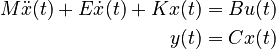
System dimensions:

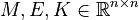$M, E, K \in \mathbb{R}^{n \times n}$, $B \in \mathbb{R}^{n \times m}$, $C \in \mathbb{R}^{p \times n}$, with $n = 779\,232$ and $m = 1$.

The internal damping is modeled as Rayleigh damping $E = \alpha_r M + \beta_r K$ using the coefficients from the table above.

System variants:

• $p = 3$: $C=$Cp in the data files,
• $p = 21$: $C=$Cp_ext in the data files.

Remarks

• Physically meaningful inputs are of dimension 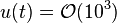$u(t) = \mathcal{O}(10^3)$. As an example, a step signal with around $5\,000$Pa leads to a horizontal POI displacement of about $3$cm.
• The interesting operation frequencies are in the range between $0$Hz and $10$Hz.
• If required, the finite element mesh behind the model and a CSV file with the output locations are available separately.
• Warning: the data files are quite large and may exceed the RAM of a typical machine if the user is also running MATLAB.

Citation

To cite this benchmark, use the following references:

• For the benchmark itself and its data:

 @Misc{SieKM19,
   author =       {Siebelts, D. and Kater, A. and Meurer, T. and Andrej, J.},
   title =        {Matrices for an Artificial Fishtail},
   howpublished = {hosted at {MORwiki} -- Model Order Reduction Wiki},
   year =         2019,
   doi =          {10.5281/zenodo.2558728}
 }

• For the background on the benchmark:

 @Article{SieKM18,
   author =       {Siebelts, D. and Kater, A. and Meurer, T.},
   title =        {Modeling and Motion Planning for an Artificial Fishtail},
   journal =      {IFAC-PapersOnLine},
   volume =       51,
   number =       2,
   year =         2018,
   pages =        {319--324},
   doi =          {10.1016/j.ifacol.2018.03.055},
   publisher =    {Elsevier {BV}}
 }

References

- ↑ D. Siebelts, A. Kater, T. Meurer, Modeling and Motion Planning for an Artificial Fishtail, IFAC-PapersOnLine (9th Vienna International Conference on Mathematical Modelling) 51(2): 319--324, 2018.