
| Line 30: | Line 30: | ||
<math> C \in \mathbb R^{p\times n}. |
<math> C \in \mathbb R^{p\times n}. |
||
</math> |
</math> |
||
| + | |||
| + | As one can see, there seems to be a close connection between LPV and bilinear systems which may be advantageous. To be more precise, we can interpret LPV systems as special bilinear system by simply setting |
||
| + | |||
| + | <math> |
||
| + | \tilde{A}=A,\;\; \tilde{N}_i=0,\;\;i=1,\dots,m,\;\; \tilde{N}_i=A_i,\;\; i=m+1,\dots,m+d, \;\; \tilde{B}=\begin{bmatrix} B_0 & 0\end{bmatrix},\;\; \tilde{C}=C, \;\; \tilde{u}=\begin{bmatrix} u_0 \\ p_1(t) \\ \vdots \\ p_d(t)\end{bmatrix} . |
||
| + | </math> |
||
| + | |||
| + | It is important to note that in this way the parameter dependency has been hidden in the structure of a bilinear systems and if we use a bilinear model reduction method, we automatically end up with a structure-preserving model reduction method for LPV systems as well. |
||
Revision as of 08:14, 6 December 2011
The model reduction method we present here is applicable to linear parameter-varying (LPV) systems of the form
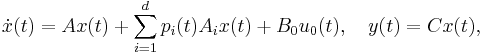
where
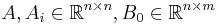 and
and

The main idea is that the structure of the above type of systems is quite similar to so-called bilinear control systems. Although belonging to the class of nonlinear control systems, the latter exhibit many features of linear time-invariant systems. In more detail, a bilinear control system is given as follows
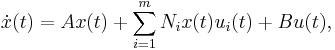
where
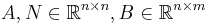 and
and
As one can see, there seems to be a close connection between LPV and bilinear systems which may be advantageous. To be more precise, we can interpret LPV systems as special bilinear system by simply setting
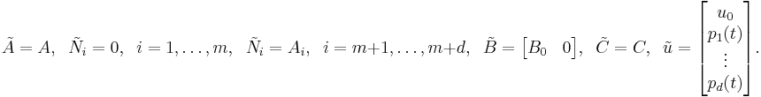
It is important to note that in this way the parameter dependency has been hidden in the structure of a bilinear systems and if we use a bilinear model reduction method, we automatically end up with a structure-preserving model reduction method for LPV systems as well.