
(init) |
|||
| Line 13: | Line 13: | ||
==Description== |
==Description== |
||
| + | A parametric semi-discretized heat transfer problem with varying heat transfer coefficients, the parameters, on subdomains. |
||
| − | |||
| + | <figure id="fig1">[[File:ThermalBlockDomain.svg|490px|thumb|right|<caption>The computational domain and boundaries.</caption>]]</figure> |
||
| + | <figure id="fig1">[[File:ThermalBlockTend.png|490px|thumb|right|<caption>A sample heat distribution at time 1.0 for parameter choice [100, 0.01, 0.001, 0.0001].</caption>]]</figure> |
||
| + | <figure id="fig1">[[File:ThermalBlockSigmaMagnitude.png|490px|thumb|right|<caption>Sigma magnitude plot of the single parameter variant.</caption>]]</figure> |
||
===Modeling=== |
===Modeling=== |
||
| + | Consider a parameter <math>\mu\in{[10^{-6},10^2]}^4\subset\mathbb{R}^{4}</math> and define the heat conductivity <math>\sigma(\xi; \mu)</math> as <math>1.0</math> when <math>\xi\in\Omega_0</math> and <math>\sigma(\xi; \mu)=\mu_i</math> when <math>\xi\in\Omega_i</math>. The heat distribution is governed by the equation: |
||
| + | :<math> |
||
| + | \partial_t \theta(t, \xi; \mu) + \nabla \cdot (- \sigma(\xi; \mu) \nabla \theta(t, \xi; \mu)) = 0,\text{ for } t\in (0,T), \text{ and } \xi \in \Omega, |
||
| + | </math> |
||
| + | with a heat-inflow condition on the left |
||
| + | :<math> |
||
| + | \sigma(\xi; \mu) \nabla \theta(t, \xi; \mu) \cdot n(\xi) = u(t)\text{ for } t \in (0,T), \text{ and } \xi \in \Gamma_{in}, |
||
| + | </math> |
||
| + | perfect isolation on the top and bottom |
||
| + | :<math> |
||
| + | \sigma(\xi; \mu) \nabla \theta(t, \xi; \mu) \cdot n(\xi) = 0\text{ for } t \in (0,T), \text{ and } \xi \in \Gamma_N, |
||
| + | </math> |
||
| + | and fixed temperature on the right |
||
| + | :<math> |
||
| + | \theta(t, \xi; \mu) = 0\text{ for } t \in (0,T), \text{ and } \xi \in \Gamma_{D}, |
||
| + | </math> |
||
| + | and initial condition |
||
| + | :<math> |
||
| + | \theta(0, \xi; \mu) = 0 \text{ for } \xi \in \Omega. |
||
| + | </math> |
||
===Discretization=== |
===Discretization=== |
||
| + | For the discretization, FENICS 2019.1 was used on a simplicial grid with first order elements. The mesh is generated from the domain specification using gmsh 3.0.6 with '<code>clscale</code>' set to <math>0.1</math>. The python based source code for the discretization can be found at Zenodo [https://doi.org/10.5281/zenodo.3691894]. |
||
| − | |||
==Origin== |
==Origin== |
||
| + | This benchmark was developed for the [https://imsc.uni-graz.at/modred2019/ MODRED 2019] proceedings. |
||
| − | |||
==Data== |
==Data== |
||
| + | The benchmark includes the basic domain description as a gmsh input file, Python scripts for the matrix assembly, simulation in pyMOR and visualization as VTK, together with the matrices both as one combined file <code>ABCE.mat</code> or separate matrix market files for all matrices. The sources and the <code>ABCE.mat</code> are available for download at [https://doi.org/10.5281/zenodo.3691894 Zenodo]. |
||
| + | Note that the heat transfer coefficients are designed as characteristic functions on the domains, such that the system is only well-posed when all entries in <math>\mu</math> positive. |
||
==Dimensions== |
==Dimensions== |
||
| + | System structure: |
||
| + | :<math> |
||
| + | \begin{align} |
||
| + | E\dot{x}(t) &= (A_0 + \mu_1 A_1 + \mu_2 A_2 + \mu_3 A_3 + \mu_4 A_4) x(t) + Bu(t), \\ |
||
| + | y(t) &= Cx(t) |
||
| + | \end{align} |
||
| + | </math> |
||
| + | |||
| + | System dimensions: |
||
| + | |||
| + | <math>E \in \mathbb{R}^{N \times N}</math>, |
||
| + | <math>A_0 \in \mathbb{R}^{N \times N}</math>, |
||
| + | <math>A_1 \in \mathbb{R}^{N \times N}</math>, |
||
| + | <math>A_2 \in \mathbb{R}^{N \times N}</math>, |
||
| + | <math>A_3 \in \mathbb{R}^{N \times N}</math>, |
||
| + | <math>A_4 \in \mathbb{R}^{N \times N}</math>, |
||
| + | <math>B \in \mathbb{R}^{N \times 1}</math>, |
||
| + | <math>C \in \mathbb{R}^{4 \times N}</math>, |
||
| + | |||
| + | where <math>N=7\,488</math> for the system matrices given in <code>ABCE.mat</code>. |
||
| + | |||
| + | ==Variants== |
||
| + | Besides the full four parameter setup, the model can be used in variations with other numbers of independent parameters. The following two are recommended in the original work and have been investigated in the literature<ref name="morBenW20c"/>,<ref name="morHim20"/>,<ref name="morBenKS20"/>. |
||
| + | |||
| + | ===one parameter=== |
||
| + | The interpretation of the thermal block as the "cookie backing" problem with slight variation in the dough leads to an easy on parameter variant. Here the new single parameter <math>\hat\mu\in [ 10^{-6}, 10^2]</math> is chosen such that <math> \mu = \hat\mu\left[0.2, 0.4, 0.6, 0.8\right]. </math> |
||
| + | |||
| + | ===Non-parametric=== |
||
| + | The system can be used as a standard LTI state space model. It is recommended to use <math>\mu = \sqrt{10} [1, 1, 1, 1]</math>. |
||
==Citation== |
==Citation== |
||
| + | To cite this benchmark, use the following references: |
||
| + | * For the benchmark itself and its data: |
||
| + | :: S. Rave and J. Saak, '''Thermal Block'''. MORwiki - Model Order Reduction Wiki, 2020. http://modelreduction.org/index.php/Thermal_Block |
||
| + | |||
| + | @MISC{morwiki_thermalblock, |
||
| + | author = <nowiki>{Rave, S. and Saak, J.}</nowiki>, |
||
| + | title = {Thermal Block}, |
||
| + | howpublished = {{MORwiki} -- Model Order Reduction Wiki}, |
||
| + | url = <nowiki>{http://modelreduction.org/index.php/Thermal_Block}</nowiki>, |
||
| + | year = 2020 |
||
| + | } |
||
| + | * For the background on the benchmark: |
||
| ⚫ | |||
| + | :: S. Rave and J. Saak, <span class="plainlinks">[https://arxiv.org/abs/2003.00846 '''An Instationary Thermal-Block Benchmark Model for Parametric Model Order Reduction''']. e-prints 2003.00846, arXiv, math.NA (2020). |
||
| + | @TECHREPORT{morRavS20, |
||
| + | author = {Rave, S. and Saak, J.}, |
||
| + | title = {An Instationary Thermal-Block Benchmark Model for Parametric |
||
| + | Model Order Reduction}, |
||
| + | institution = {arXiv}, |
||
| + | type = {e-print}, |
||
| + | number = {2003.00846}, |
||
| + | note = {math.NA}, |
||
| + | year = 2020, |
||
| + | url = <nowiki>{https://arxiv.org/abs/2003.00846}</nowiki> |
||
| + | } |
||
| + | |||
| ⚫ | |||
| + | <references> |
||
| + | <ref name="morBenW20c">P. Benner, S. W. R. Werner, <span class="plainlinks">[https://arxiv.org/abs/2002.12682 MORLAB – the Model Order Reduction LABoratory], |
||
| + | e-print 2002.12682, arXiv, cs.MS (2020).</ref> |
||
| + | <ref name="morHim20">C. Himpe, <span class="plainlinks">[https://arxiv.org/abs/2002.12226 Comparing (empirical-Gramian-based) model order reduction algorithms], e-prints 2002.12226, arXiv, math.OC (2020).</ref> |
||
| + | <ref name="morBenKS20">P. Benner, M. Köhler, J. Saak, <span class="plainlinks">[https://arxiv.org/abs/2003.02088 Matrix equations, sparse solvers: M-M.E.S.S.-2.0.1 – philosophy, features and application for (parametric) model order reduction], eprints 2003.02088, arXiv, cs.MS (2020).</ref> |
||
| + | </references> |
||
==Contact== |
==Contact== |
||
| + | '' [[User:Saak]]'' |
||
Revision as of 17:23, 10 March 2020
 Note: This page has not been verified by our editors.
Description
A parametric semi-discretized heat transfer problem with varying heat transfer coefficients, the parameters, on subdomains.


Modeling
Consider a parameter ![\mu\in{[10^{-6},10^2]}^4\subset\mathbb{R}^{4}](/morwiki/images/math/b/0/5/b055bfc56b41ae34dc4343ace56270d7.png) and define the heat conductivity
and define the heat conductivity  as
as  when
when  and
and  when
when  . The heat distribution is governed by the equation:

with a heat-inflow condition on the left

perfect isolation on the top and bottom

and fixed temperature on the right

and initial condition
Discretization
For the discretization, FENICS 2019.1 was used on a simplicial grid with first order elements. The mesh is generated from the domain specification using gmsh 3.0.6 with 'clscale' set to  . The python based source code for the discretization can be found at Zenodo [1].
Origin
This benchmark was developed for the MODRED 2019 proceedings.
Data
The benchmark includes the basic domain description as a gmsh input file, Python scripts for the matrix assembly, simulation in pyMOR and visualization as VTK, together with the matrices both as one combined file ABCE.mat or separate matrix market files for all matrices. The sources and the ABCE.mat are available for download at Zenodo.
Note that the heat transfer coefficients are designed as characteristic functions on the domains, such that the system is only well-posed when all entries in  positive.
Dimensions
System structure:
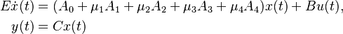
System dimensions:
 ,
,
 ,
,
 ,
,
 ,
,
 ,
,
 ,
,
 ,
,
 ,
,
where  for the system matrices given in
 ABCE.mat.
Variants
Besides the full four parameter setup, the model can be used in variations with other numbers of independent parameters. The following two are recommended in the original work and have been investigated in the literature[1],[2],[3].
one parameter
The interpretation of the thermal block as the "cookie backing" problem with slight variation in the dough leads to an easy on parameter variant. Here the new single parameter ![\hat\mu\in [ 10^{-6}, 10^2]](/morwiki/images/math/7/8/e/78e442ccec98fe42c3cfe7078f053362.png) is chosen such that
is chosen such that ![\mu = \hat\mu\left[0.2, 0.4, 0.6, 0.8\right].](/morwiki/images/math/9/1/0/91066c3fba0a3c4e85098ec997d69808.png)
Non-parametric
The system can be used as a standard LTI state space model. It is recommended to use ![\mu = \sqrt{10} [1, 1, 1, 1]](/morwiki/images/math/2/2/6/2265244b5bc1beaf0212762bc19d20a1.png) .
.
Citation
To cite this benchmark, use the following references:
- For the benchmark itself and its data:
- S. Rave and J. Saak, Thermal Block. MORwiki - Model Order Reduction Wiki, 2020. http://modelreduction.org/index.php/Thermal_Block
@MISC{morwiki_thermalblock,
  author =       {Rave, S. and Saak, J.},
  title =        {Thermal Block},
  howpublished = {{MORwiki} -- Model Order Reduction Wiki},
  url =          {http://modelreduction.org/index.php/Thermal_Block},
  year =         2020
}
- For the background on the benchmark:
- S. Rave and J. Saak, An Instationary Thermal-Block Benchmark Model for Parametric Model Order Reduction. e-prints 2003.00846, arXiv, math.NA (2020).
@TECHREPORT{morRavS20,
  author =       {Rave, S. and Saak, J.},
  title =        {An Instationary Thermal-Block Benchmark Model for Parametric
                  Model Order Reduction},
  institution =  {arXiv},
  type =         {e-print},
  number =       {2003.00846},
  note =         {math.NA},
  year =         2020,
  url =          {https://arxiv.org/abs/2003.00846}
}
References
- ↑ P. Benner, S. W. R. Werner, MORLAB – the Model Order Reduction LABoratory, e-print 2002.12682, arXiv, cs.MS (2020).
- ↑ C. Himpe, Comparing (empirical-Gramian-based) model order reduction algorithms, e-prints 2002.12226, arXiv, math.OC (2020).
- ↑ P. Benner, M. Köhler, J. Saak, Matrix equations, sparse solvers: M-M.E.S.S.-2.0.1 – philosophy, features and application for (parametric) model order reduction, eprints 2003.02088, arXiv, cs.MS (2020).