(init Stokes) |
(Stokes description init) |
||
| Line 1: | Line 1: | ||
{{preliminary}} <!-- Do not remove --> |
{{preliminary}} <!-- Do not remove --> |
||
| + | |||
| + | [[Category:benchmark]] |
||
| + | [[Category:procedural]] |
||
| + | [[Category:SISO]] |
||
[[Category:linear]] |
[[Category:linear]] |
||
| + | [[Category:Sparse]] |
||
==Description== |
==Description== |
||
| + | This benchmark presents the two-dimensional instationary [[wikipedia:Stokes_flow|Stokes equation]], |
||
| + | which models flow of an incompressible fluid in a domain. |
||
| + | The associated partial differential equation system is given by: |
||
| + | :<math> |
||
| + | \begin{align} |
||
| + | \frac{\partial v}{\partial t} &= \Delta v - \nabla p + f, \qquad (x,t) \in \Omega \times (0,T] \\ |
||
| + | 0 &= \operatorname{div} v, \\ |
||
| + | v &= 0, \qquad \qquad \qquad \quad \; (x,t) \in \partial \Omega \times (0,T] |
||
| + | \end{align} |
||
| + | </math> |
||
| + | with velocity variable <math>v(x,t)</math> and pressure variable <math>\rho(x,t)</math>, |
||
| + | on a spatial domain <math>\Omega = [0,1] \times [0,1] \subset \mathbb{R}^2</math>, |
||
| + | and an external forcing term <math>f</math>. |
||
| + | The boundary conditions are no-slip. |
||
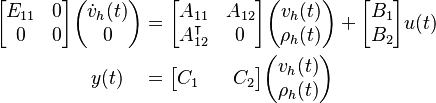
| + | A finite difference discretization yields the descriptor system: |
||
| − | |||
| + | :<math> |
||
| + | \begin{align} |
||
| + | \begin{bmatrix} E_{11} & 0 \\ 0 & 0 \end{bmatrix} \begin{pmatrix} \dot{v}_h(t) \\ 0 \end{pmatrix} &= |
||
| + | \begin{bmatrix} A_{11} & A_{12} \\ A_{12}^\intercal & 0 \end{bmatrix} \begin{pmatrix} v_h(t) \\ \rho_h(t) \end{pmatrix} + |
||
| + | \begin{bmatrix} B_1 \\ B_2 \end{bmatrix} u(t) \\ |
||
| + | y(t)\quad & = \begin{bmatrix} C_1 \,\;&\;\, C_2 \end{bmatrix} \begin{pmatrix} v_h(t) \\ \rho_h(t) \end{pmatrix} |
||
| + | \end{align} |
||
| + | </math> |
||
| + | The matrix <math>A_{11}</math> matrix is the discretized Laplace operator, |
||
| + | while <math>A_{12}</math> corresponds to the discrete gradient and divergence operators. |
||
| + | For this benchmark the compound discretization of the boundary values and external forcing <math>[B_1 \; B_2]^\intercal \in \mathbb{R}^{N \times 1}</math> is chosen (uniformly) randomly, |
||
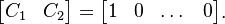
| + | whereas the output matrix <math>[C_1 \; C_2] \in \mathbb{R}^{1 \times N}</math> is set to: |
||
| + | :<math> |
||
| + | \begin{align} |
||
| + | \begin{bmatrix} C_1 & C_2 \end{bmatrix} = \begin{bmatrix} 1 & 0 & \dots & 0 \end{bmatrix}. |
||
| + | \end{align} |
||
| + | </math> |
||
==Origin== |
==Origin== |
||
Revision as of 09:08, 26 June 2019
 Note: This page has not been verified by our editors.
Description
This benchmark presents the two-dimensional instationary Stokes equation, which models flow of an incompressible fluid in a domain. The associated partial differential equation system is given by:
![\begin{align}
\frac{\partial v}{\partial t} &= \Delta v - \nabla p + f, \qquad (x,t) \in \Omega \times (0,T] \\
0 &= \operatorname{div} v, \\
v &= 0, \qquad \qquad \qquad \quad \; (x,t) \in \partial \Omega \times (0,T]
\end{align}](/morwiki/images/math/0/f/2/0f27e911ee5f720dc7a92df241bc09ed.png)
with velocity variable  and pressure variable
  ,
on a spatial domain
,
on a spatial domain ![\Omega = [0,1] \times [0,1] \subset \mathbb{R}^2](/morwiki/images/math/5/2/a/52a66b1b7e6a3db2aef33f4c13f8c98a.png) ,
and an external forcing term
,
and an external forcing term  .
The boundary conditions are no-slip.
.
The boundary conditions are no-slip.
A finite difference discretization yields the descriptor system:
The matrix  matrix is the discretized Laplace operator,
while
matrix is the discretized Laplace operator,
while  corresponds to the discrete gradient and divergence operators.
For this benchmark the compound discretization of the boundary values and external forcing
corresponds to the discrete gradient and divergence operators.
For this benchmark the compound discretization of the boundary values and external forcing ![[B_1 \; B_2]^\intercal \in \mathbb{R}^{N \times 1}](/morwiki/images/math/a/7/4/a74f83a828f5633b306d840d266ff230.png) is chosen (uniformly) randomly,
whereas the output matrix
is chosen (uniformly) randomly,
whereas the output matrix ![[C_1 \; C_2] \in \mathbb{R}^{1 \times N}](/morwiki/images/math/4/1/9/419c80fae8155eae9c868bef71fdbe5b.png) is set to:
is set to: