
(init) |
(more content) |
||
| Line 23: | Line 23: | ||
===First Order Representation=== |
===First Order Representation=== |
||
| + | |||
| + | The second order system can be represented as a first order system as follows: |
||
:<math> |
:<math> |
||
| Line 28: | Line 30: | ||
\begin{pmatrix} 1 & 0 \\ 0 & M \end{pmatrix} \begin{pmatrix} \dot{p} \\ \dot{v} \end{pmatrix} &= |
\begin{pmatrix} 1 & 0 \\ 0 & M \end{pmatrix} \begin{pmatrix} \dot{p} \\ \dot{v} \end{pmatrix} &= |
||
\begin{pmatrix} 0 & 1 \\ K & D \end{pmatrix} \begin{pmatrix} p \\ v \end{pmatrix} + |
\begin{pmatrix} 0 & 1 \\ K & D \end{pmatrix} \begin{pmatrix} p \\ v \end{pmatrix} + |
||
| − | \begin{pmatrix} 0 \\ |
+ | \begin{pmatrix} 0 \\ f_p(p) \end{pmatrix} + \begin{pmatrix} 0 \\ B_v \end{pmatrix} \\ |
| − | y &= \begin{pmatrix} |
+ | y &= \begin{pmatrix} C_p & 0 \end{pmatrix} \begin{pmatrix} p \\ v \end{pmatrix} |
\end{align} |
\end{align} |
||
</math> |
</math> |
||
| + | |||
| + | with the components: |
||
:<math> |
:<math> |
||
| − | M = m \begin{pmatrix} 1 \\ & \ddots \end{pmatrix} |
+ | M = m \begin{pmatrix} 1 \\ & \ddots \end{pmatrix}, \quad |
| − | + | K_0 = k_l \begin{pmatrix} -2 & 1 \\ 1 & -2 & \ddots \\ & \ddots & \ddots \end{pmatrix}, \quad |
|
D = d \begin{pmatrix} -2 & 1 \\ 1 & -2 & \ddots \\ & \ddots & \ddots \end{pmatrix}, \quad |
D = d \begin{pmatrix} -2 & 1 \\ 1 & -2 & \ddots \\ & \ddots & \ddots \end{pmatrix}, \quad |
||
| − | + | B_v = \begin{pmatrix} 0 \\ \vdots \\ 0 \\ 1 \end{pmatrix}, \quad |
|
| − | + | C_p = \begin{pmatrix} 0 & \dots & 0 & 1 \end{pmatrix}, |
|
| ⚫ | |||
</math> |
</math> |
||
| + | |||
| + | and the nonlinear term: |
||
| + | |||
| + | :<math> |
||
| ⚫ | |||
| + | </math> |
||
| + | |||
| + | and thus yielding the classic first order components: |
||
| + | |||
| + | :<math> |
||
| + | E = \begin{pmatrix} 1 & 0 \\ 0 & M \end{pmatrix}, \quad |
||
| + | A = \begin{pmatrix} 0 & 1 \\ K & D \end{pmatrix}, \quad |
||
| + | B = \begin{pmatrix} 0 \\ B_v \end{pmatrix}, \quad |
||
| + | C = \begin{pmatrix} C_p & 0 \end{pmatrix}. |
||
| + | </math> |
||
| + | |||
| + | The parameters for the mass <math>m</math>, linear spring constant <math>k_l</math>, nonlinear spring constant <math>k_n</math>, and damping <math>d</math> are chosen in <ref name="kawano15"/> as <math>m=1</math>, <math>k_l=1</math>, <math>k_n=2</math>, and <math>d=1</math>. |
||
==Data== |
==Data== |
||
| + | The following Matlab code assembles the above described <math>E</math>, <math>A</math>, <math>B</math> and <math>C</math> parameter dependent matrices and the function <math>f</math> for a given number of subsystems <math>N</math>. |
||
| + | |||
| + | <div class="thumbinner" style="width:540px;text-align:left;"> |
||
| + | <source lang="matlab"> |
||
| + | function [E,A,B,C,f] = msd(N) |
||
| + | |||
| + | U = speye(N); % Sparse unit matrix |
||
| + | T = gallery('tridiag',N,-1,2,-1); % Sparse tridiagonal matrix |
||
| + | H = gallery('tridiag',N,-1,1,0); % Sparse transport matrix |
||
| + | Z = sparse(N,N); % Sparse all zero matrix |
||
| + | z = sparse(N,1); % Sparse all zero vector |
||
| + | |||
| + | E = @(m) [U,Z;Z,m*U]; % Handle to parametric E matrix |
||
| + | A = @(kl,d) [Z,U;kl*T,d*T]; % Handle to parametric A matrix |
||
| + | B = sparse(2*N,1,1,2*N,1); |
||
| + | C = sparse(N,1,1,2*N,1); |
||
| + | f = @(x,kn) [z;-kn*( (H'*x(N+1:end)).^3 - (H*x(N+1:end)).^3)]; |
||
| + | end |
||
| + | </source> |
||
| + | </div> |
||
| Line 51: | Line 91: | ||
System structure: |
System structure: |
||
| + | :<math> |
||
| + | \begin{array}{rcl} |
||
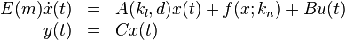
| + | E(m) \dot{x}(t) &=& A(k_l,d)x(t) + f(x;k_n) + Bu(t) \\ |
||
| + | y(t) &=& Cx(t) |
||
| + | \end{array} |
||
| + | </math> |
||
| + | |||
| + | System dimensions: |
||
| + | <math>E \in \mathbb{R}^{2N \times 2N}</math>, |
||
| + | <math>A \in \mathbb{R}^{2N \times 2N}</math>, |
||
| + | <math>B \in \mathbb{R}^{2N \times 1}</math>, |
||
| + | <math>C \in \mathbb{R}^{1 \times 2N}</math>. |
||
==Citation== |
==Citation== |
||
| Line 80: | Line 132: | ||
doi = {10.1007/978-3-319-20988-3} |
doi = {10.1007/978-3-319-20988-3} |
||
} |
} |
||
| − | |||
==References== |
==References== |
||
| Line 89: | Line 140: | ||
</references> |
</references> |
||
| − | |||
| − | |||
| − | ==Contact== |
||
| − | |||
| − | [[User:Himpe]] |
||
Revision as of 14:14, 11 December 2018
 Note: This page has not been verified by our editors.
Description: Mass-Spring-Damper System
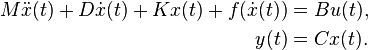
This benchmark is a generalization of the nonlinear mass-spring-damper system presented in [1], which is concerned with modeling the a mechanical systems consisting of chained masses, linear and nonlinear springs, and dampers. The underlying mathematical model is a second order system:
First Order Representation
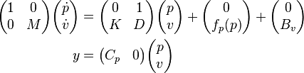
The second order system can be represented as a first order system as follows:
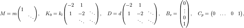
with the components:
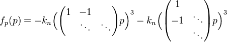
and the nonlinear term:
and thus yielding the classic first order components:

The parameters for the mass  , linear spring constant
  , nonlinear spring constant
  , and damping
  are chosen in [1] as
  ,
,  ,
,  , and
, and  .
.
Data
The following Matlab code assembles the above described  ,
,  ,
,  and
and  parameter dependent matrices and the function
  for a given number of subsystems
  .
.
function [E,A,B,C,f] = msd(N)

    U = speye(N);                     % Sparse unit matrix
    T = gallery('tridiag',N,-1,2,-1); % Sparse tridiagonal matrix
    H = gallery('tridiag',N,-1,1,0);  % Sparse transport matrix
    Z = sparse(N,N);                  % Sparse all zero matrix
    z = sparse(N,1);                  % Sparse all zero vector

    E = @(m) [U,Z;Z,m*U];             % Handle to parametric E matrix
    A = @(kl,d) [Z,U;kl*T,d*T];       % Handle to parametric A matrix
    B = sparse(2*N,1,1,2*N,1);
    C = sparse(N,1,1,2*N,1);
    f = @(x,kn) [z;-kn*( (H'*x(N+1:end)).^3 - (H*x(N+1:end)).^3)];
end
Dimensions
System structure:
System dimensions:
 ,
,
 ,
,
 ,
,
 .
.
Citation
To cite this benchmark, use the following references:
- For the benchmark itself and its data:
- The MORwiki Community, Mass-Spring-Damper System. MORwiki - Model Order Reduction Wiki, 2018. http://modelreduction.org/index.php/Mass-Spring-Damper
@MISC{morwiki_msd,
  author =       {{The MORwiki Community}},
  title =        {Mass-Spring-Damper System},
  howpublished = {hosted at {MORwiki} -- Model Order Reduction Wiki},
  url =          {http://modelreduction.org/index.php/Mass-Spring-Damper},
  year =         2018
}
- For the background on the benchmark:
@INPROCEEDINGS{morKawS15,
  title =        {Model Reduction by Generalized Differential Balancing},
  author =       {Y. Kawano and J.M.A. Scherpen},
  booktitle =    {Mathematical Control Theory I: Nonlinear and Hybrid Control Systems},
  series =       {Lecture Notes in Control and Information Sciences},
  volume =       {461},
  pages =        {349--362},
  year =         {2015},
  doi =          {10.1007/978-3-319-20988-3}
}
References
- ↑ 1.0 1.1 Y. Kawano and J.M.A. Scherpen, Model Reduction by Generalized Differential Balancing, In: Mathematical Control Theory I: Nonlinear and Hybrid Control Systems, Lecture Notes in Control and Information Sciences 461: 349--362, 2015.