FitzHugh-Nagumo System

Description

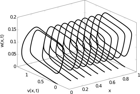
The FitzHugh-Nagumo system describes a prototype of an excitable system, e.g., a neuron. If the external stimulus $i_0(t)$ exceeds a certain threshold value, the system will exhibit a characteristic excursion in phase space, before the variables $v$ and $w$ relax back to their rest values. This behaviour is typical for spike generations (=short elevation of membrane voltage $v$) in a neuron after stimulation by an external input current.

Figure 1: FitzHugh-Nagumo System

Here, we present the setting from , where the equations for the dynamical system read

$\epsilon v_t(x,t)=\epsilon^2v_{xx}(x,t)+f(v(x,t))-w(x,t)+g,$

$w_t(x,t)=hv(x,t)-\gamma w(x,t)+g,$

with $f(v)=v(v-0.1)(1-v)$ and initial and boundary conditions

$v(x,0)=0,\quad w(x,0)=0, \quad x\in [0,1],$

$v_x(0,t)=-i_0(t), \quad v_x(1,t)\quad =0, \quad t \geq 0,$

where $\epsilon=0.015,\;h=0.5,\;\gamma=2,\;g=0.05,\;i_0(t)=5\cdot 10^4t^3 \exp(-15t).$ In , the previous system of coupled nonlinear PDEs is spatially discretized by means of a finite difference scheme with $k=512$ nodes for each PDE. Hence, one obtains a nonlinear (cubic) system of ODEs with state dimension $n=1024$. xx--CrossReference--dft--fig:fhn--xx shows the typical limit cycle behaviour described above.

Reformulation as a quadratic-bilinear system

Instead of the cubic system of ODEs, one can alternatively study a so-called quadratic-bilinear control system of the form

$E\dot{x}(t) = A x(t) + H x(t) \otimes x(t) + N x(t) u(t) + b u(t),$

with $E,A,N \in \mathbb R^{n\times n},\ H \in \mathbb R^{n\times n^2}$ and $b \in \mathbb R.$ The idea relies on artificially introducing a new state variable defined as $z(t)=v(t)^2$ and subsequently computing the dynamics of the new variable, i.e., specifying $\dot{z}(t).$ The technique goes back to , where it is successfully applied to several smooth nonlinear control-affine systems. As it is discussed in , the previously mentioned introduction of $z$ yields a quadratic-bilinear control of dimension $N = 3\cdot k$ with state vector $x = [v,w,z]^T.$ The increase of the state dimension has the advantage of reducing the nonlinearity from cubic to quadratic. This however opens up the possibility to reduce the system by the generalized moment-matching approach from , see also for more details on the implementation.

Data

All matrices of the quadratic-bilinear formulation discretized with $k=512$ are in the Matrix Market format. The matrix name is used as an extension of the matrix file and can be found at:

FitzNagumo.tar.gz.

For the input function, we have $u(t)=[i_0(t),1]$. For more information on the discretization details, see .

Contact

Tobias Breiten

References

- ↑ 1.0 1.1 1.2 S. Chaturantabut and D.C. Sorensen, "Nonlinear Model Reduction via Discrete Empirical Interpolation", SIAM J. Sci. Comput., 32 (2010), pp. 2737-2764.
- ↑ 2.0 2.1 C. Gu, "QLMOR: A Projection-Based Nonlinear Model Order Reduction Approach Using Quadratic-Linear Representation of Nonlinear Systems", IEEE T. Comput. Aid. D., 30 (2011), pp. 1307-1320.
- ↑ 3.0 3.1 P. Benner and T. Breiten, "Two-sided Moment Matching Methods for Nonlinear Model Eeduction", 2012, Preprint MPIMD/12-12.
![v(x,0)=0,\quad w(x,0)=0, \quad x\in [0,1],](/morwiki/images/math/a/4/6/a46a8b06dcccd3bdbb094e4acad72a28.png)