
(Init FSS Benchmark) |
m (Fix tex errors) |
||
| Line 13: | Line 13: | ||
In modal form the '''flexible space structure''' model for <math>K</math> modes, <math>M</math> actuators and <math>Q</math> sensors is of second order and given by: |
In modal form the '''flexible space structure''' model for <math>K</math> modes, <math>M</math> actuators and <math>Q</math> sensors is of second order and given by: |
||
| + | |||
| − | :<math> |
||
| − | \ddot{\nu}(t) |
+ | :<math>\ddot{\nu}(t) = (2 \xi \circ \omega) \circ \dot{\nu}(t) + (\omega \circ \omega) \circ \nu = Bu(t)</math> |
| + | |||
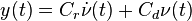
| − | + | :<math>y(t) = C_r\dot{\nu}(t) + C_d\nu(t)</math> |
|
| − | </math> |
||
| + | |||
| − | with the parameters <math>\xi \in \mathbb{R}_{>0}^K</math> (damping ratio), <math>\omega \in \mathbb{R}_{>0}^K</math> (natural frequency) and using the Hadamard product |
+ | with the parameters <math>\xi \in \mathbb{R}_{>0}^K</math> (damping ratio), <math>\omega \in \mathbb{R}_{>0}^K</math> (natural frequency) and using the Hadamard product <math>\circ</math>. |
| − | The first order representation follows for <math>x(t) = (\dot{nu}(t), \omega_1\nu_1, \dots, \omega_K\nu_K)</math> by: |
+ | The first order representation follows for <math>x(t) = (\dot{\nu}(t), \omega_1\nu_1, \dots, \omega_K\nu_K)</math> by: |
| − | :<math> |
||
| + | |||
| − | \dot{x}(t) &= Ax(t) + Bu(t) \\ |
||
| − | + | :<math>\dot{x}(t) = Ax(t) + Bu(t) </math> |
|
| + | |||
| − | </math> |
||
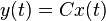
| + | :<math>y(t) = Cx(t)</math> |
||
| + | |||
with the matrices: |
with the matrices: |
||
| + | |||
| − | :<math> |
||
| − | A := \begin{pmatrix} A_1 & & \\ & \ddots & \\ & & A_K \end{pmatrix}, \\ |
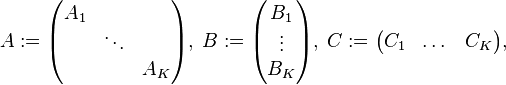
+ | :<math>A := \begin{pmatrix} A_1 & & \\ & \ddots & \\ & & A_K \end{pmatrix}, \; B := \begin{pmatrix} B_1 \\ \vdots \\ B_K \end{pmatrix}, \; C := \begin{pmatrix} C_1 & \dots & C_K \end{pmatrix}, </math> |
| + | |||
| − | B := \begin{pmatrix} B_1 \\ \vdots \\ B_K \end{pmatrix}, \\ |
||
| − | C := \begin{pmatrix} C_1 & \dots & C_K \end{pmatrix}, |
||
| − | </math> |
||
and their components: |
and their components: |
||
| + | |||
| − | :<math> |
||
| − | A_k := \begin{pmatrix} -2\xi_k\omega_k & -\omega_k \\ \omega_k & 0 \end{pmatrix}, \\ |
+ | :<math>A_k := \begin{pmatrix} -2\xi_k\omega_k & -\omega_k \\ \omega_k & 0 \end{pmatrix}, \; B_k := \begin{pmatrix} b_k \\ 0 \end{pmatrix}, \; C_k := \begin{pmatrix} c_{rk} & \frac{c_{dk}}{\omega_k} \end{pmatrix},</math> |
| + | |||
| − | B_k := \begin{pmatrix} b_k \\ 0 \end{pmatrix}, \\ |
||
| − | C_k := \begin{pmatrix} c_{rk} & \frac{c_{dk}}{\omega_k} \end{pmatrix}, |
||
| − | </math> |
||
where <math>b_k \in \mathbb{R}^{1 \times M}</math> and <math>c_{rk}, c_{dk} \in \mathbb{R}^{Q \times 1}</math>. |
where <math>b_k \in \mathbb{R}^{1 \times M}</math> and <math>c_{rk}, c_{dk} \in \mathbb{R}^{Q \times 1}</math>. |
||
| Line 41: | Line 39: | ||
For this benchmark the system matrix is block diagonal and thus chosen to be sparse. |
For this benchmark the system matrix is block diagonal and thus chosen to be sparse. |
||
| − | The parameters <math>\xi</math> and math>\omega</math> are sampled from a uniform random distributions <math>\mathcal{U}_[0,\frac{1}{1000}]}^K</math> and <math>\mathcal{U}_[0,100]}^K</math> respectively. |
+ | The parameters <math>\xi</math> and math>\omega</math> are sampled from a uniform random distributions <math>\mathcal{U}_{[0,\frac{1}{1000}]}^K</math> and <math>\mathcal{U}_{[0,100]}^K</math> respectively. |
The components of the input matrix <math>b_k</math> are sampled form a uniform random distribution <math>\mathcal{U}_{[0,1]}</math>, |
The components of the input matrix <math>b_k</math> are sampled form a uniform random distribution <math>\mathcal{U}_{[0,1]}</math>, |
||
while the output matrix <math>C</math> is sampled from a uniform random distribution <math>\mathcal{U}^{}_[0,10]</math> completely w.l.o.g, since if the components of <math>C_d</math> are random their scaling can be ignored. |
while the output matrix <math>C</math> is sampled from a uniform random distribution <math>\mathcal{U}^{}_[0,10]</math> completely w.l.o.g, since if the components of <math>C_d</math> are random their scaling can be ignored. |
||
Revision as of 11:01, 11 May 2017
 Note: This page has not been verified by our editors.
Description
The flexible space structure benchmark[1] is a procedural modal model which represents structural dynamics with a selectable number actuators and sensors.
Model
In modal form the flexible space structure model for  modes,
  actuators and
  sensors is of second order and given by:

with the parameters  (damping ratio),
  (natural frequency) and using the Hadamard product
  .
The first order representation follows for
.
The first order representation follows for  by:
by:

with the matrices:
and their components:
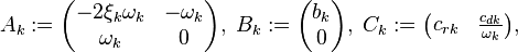
where  and
and  .
.
Benchmark Specifics
For this benchmark the system matrix is block diagonal and thus chosen to be sparse.
The parameters  and math>\omega</math> are sampled from a uniform random distributions
 ![\mathcal{U}_{[0,\frac{1}{1000}]}^K](/morwiki/images/math/2/4/b/24b74811b308c537765802cb07a302f7.png) and
and ![\mathcal{U}_{[0,100]}^K](/morwiki/images/math/3/4/2/342f256255fdd3d862d8d938a73b7d07.png) respectively.
The components of the input matrix
respectively.
The components of the input matrix  are sampled form a uniform random distribution
 ![\mathcal{U}_{[0,1]}](/morwiki/images/math/8/9/1/8914ff20760d02f585b13a7a84bf17e7.png) ,
while the output matrix
,
while the output matrix  is sampled from a uniform random distribution
 ![\mathcal{U}^{}_[0,10]](/morwiki/images/math/3/9/9/399ba46973f16420bd6eed7c2dc9e965.png) completely w.l.o.g, since if the components of
completely w.l.o.g, since if the components of  are random their scaling can be ignored.
Data
The following Matlab code assembles the above described  ,
,  and matrix for a given number of modes .
function [A,B,C] = fss(K,M,Q)

    rand('seed',1009);
    xi = rand(1,K)*0.001;	% Sample damping ratio
    omega = rand(1,K)*100;	% Sample natural frequencies

    A_k = cellfun(@(p) sparse([-2.0*p(1)*p(2),-p(2);p(2),0]), ...
                  num2cell([xi;omega],1),'UniformOutput',0);

    A = blkdiag(A_k{:});

    B = kron(rand(K,M),[1;0]);

    C = 10.0*rand(Q,2*K);
end
Reference
- ↑ W. Gawronski and T. Williams, "Model Reduction for Flexible Space Structures", Journal of Guidance 14(1): 68--76, 1991