Nonlinear RC Ladder

Description

The nonlinear RC-ladder is an electronic test circuit introduced in. This nonlinear first-order system models a resistor-capacitor network that exhibits a distinct nonlinear behaviour caused by the nonlinear resistors consisting of a parallel connected resistor with a diode.

Nonlinear RC-Ladder

Model

The underlying model is given by a (SISO) gradient system of the form:

$\dot{x}(t) = \begin{pmatrix} -g(x_1(t)) - g(x_1(t) - x_2(t)) \\ g(x_1(t)-x_2(t)) - g(x_2(t)-x_3(t)) \\ \vdots \\ g(x_{k-1}(t) - x_k(t)) - g(x_k(t) - x_{x+1}(t)) \\ \vdots \\ g(x_{N-1}(t) - x_N(t)) \end{pmatrix}+\begin{pmatrix}u(t) \\ 0 \\ \vdots \\ 0 \\ \vdots \\ 0 \end{pmatrix},$

$y(t) = x_1(t),$

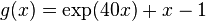
where the nonlinearity $g(x):\mathbb{R} \to \mathbb{R}$ is given by:

$g(x) = \exp(40x) + x - 1$

Input

As external input several alternatives are presented in, which are listed next. A simple step function is given by:

$u_1(t)=\begin{cases}0 & t < 4 \\ 1 & t \geq 4 \end{cases},$

an exponential decaying input is provided by:

$u_2(t) = e^{-t}.$

Additional input sources are given by conjunction of sine waves with different periods:

$u_3(t) = \sin(2\pi 50t)+\sin(2\pi 1000t),$

$u_4(t) = \sin(2\pi 50t) \sin(2\pi 1000t).$

Data

A sample procedural MATLAB implementation of order N is given by:

%% Procedural generation of "Nonlinear RC Ladder" benchmark system

% nonlinearity
g = @(x) exp(40.0*x) + x - 1.0;

A0 = sparse(N,N);
A0(1,1) = 1;

A1 = spdiags(ones(N-1,1),-1,N,N) - speye(N);
A1(1,1) = 0;

A2 = spdiags([ones(N-1,1);0],0,N,N) - spdiags(ones(N,1),1,N,N);

% input matrix
B = sparse(N,1);
B(1,1) = 1;

% output matrix
C = sparse(1,N);
C(1,1) = 1;

% vector field and output functional
xdot = @(x) -g(A0*x) + g(A1*x) - g(A2*x) + B*u;
   y = @(x) C*x;

Contact

Christian Himpe

References

- ↑ Y. Chen, "Model Reduction for Nonlinear Systems", Master Thesis, 1999.
- ↑ Y. Chen and J. White, "A quadratic method for nonlinear model order reduction", Int. conference on modelling and simulation of Microsystems semiconductors, sensors and actuators, 2000.
- ↑ M. Condon and R. Ivanov, "Empirical balanced truncation for nonlinear systems", Journal of Nonlinear Science 14(5):405--414, 2004.
- ↑ M. Condon and R. Ivanov, "Model Reduction of Nonlinear Systems", COMPEL 23(2): 547--557, 2004