
(direct truncation paragraph) |
(change BT to BT for systems in generalized state space form) |
||
| Line 8: | Line 8: | ||
==Derivation == |
==Derivation == |
||
| + | We consider linear time-invariant systems, defined in generalized state-space form by |
||
| ⚫ | |||
| − | <math> \dot{x} = Ax + Bu</math> |
+ | <math> E\dot{x} = Ax + Bu,</math> |
| − | <math> y = Cx + Du</math> |
+ | <math> y = Cx + Du,</math> |
| + | where nonsingularity of <math>E</math> and stability (<math>A - \lambda E</math> stable) is assumed. |
||
| ⚫ | is called balanced<ref>B.C. Moore, "<span class="plainlinks">[http://dx.doi.org/10.1109/TAC.1981.1102568 Principal component analysis in linear systems: Controllability, observability, and model reduction]</span>", IEEE Transactions on Automatic Control , vol.26, no.1, pp.17,32, Feb 1981</ref>, if the systems [[wikipedia:Controllability_Gramian|Controllability Gramian]] and [[wikipedia:Observability_Gramian|Observability Gramian]], the solutions <math>W_C</math> and <math>W_O</math> of the Lyapunov equations |
||
| ⚫ | |||
| ⚫ | |||
| − | <math> A^TW_O+W_OA=-C^TC </math> |
||
| ⚫ | is called balanced<ref>B.C. Moore, "<span class="plainlinks">[http://dx.doi.org/10.1109/TAC.1981.1102568 Principal component analysis in linear systems: Controllability, observability, and model reduction]</span>", IEEE Transactions on Automatic Control , vol.26, no.1, pp.17,32, Feb 1981</ref>, if the systems [[wikipedia:Controllability_Gramian|Controllability Gramian]] and [[wikipedia:Observability_Gramian|Observability Gramian]], i.e. the solutions <math>W_C</math> and <math>W_O</math> of the (generalized) Lyapunov equations |
||
| ⚫ | |||
| ⚫ | |||
| + | |||
| + | <math> A^T\hat W_OE+E^T\hat W_OA=-C^TC, \quad W_O=E^T\hat W_O E, </math> |
||
| + | |||
| ⚫ | |||
Since in general, the spectrum of <math>W_CW_O</math> are the squared Hankel Singular Values for such a balanced system, they are given by: <math>\sqrt{\lambda(W_CW_O)} = \{\sigma_1,\dots,\sigma_n\}</math>. |
Since in general, the spectrum of <math>W_CW_O</math> are the squared Hankel Singular Values for such a balanced system, they are given by: <math>\sqrt{\lambda(W_CW_O)} = \{\sigma_1,\dots,\sigma_n\}</math>. |
||
| − | An arbitrary system <math>(A,B,C,D)</math> can be transformed into a balanced system <math>(\tilde{A},\tilde{B},\tilde{C},\tilde{D})</math> via a state-space transformation: |
+ | An arbitrary system <math>(E,A,B,C,D)</math> can be transformed into a balanced system <math>(\tilde{E},\tilde{A},\tilde{B},\tilde{C},\tilde{D})</math> via a state-space transformation: |
| − | <math> (\tilde{A},\tilde{B},\tilde{C},\tilde{D})= (TAT^{-1},TB,CT^{-1},D).</math> |
+ | <math> (\tilde{E},\tilde{A},\tilde{B},\tilde{C},\tilde{D})= (TET^{-1},TAT^{-1},TB,CT^{-1},D).</math> |
This transformed system has balanced Gramians <math>W_C=T\tilde{W_C}T^T</math> and <math>W_O=T^{-T}\tilde{W_O}T^{-1}</math> which are equal and diagonal. |
This transformed system has balanced Gramians <math>W_C=T\tilde{W_C}T^T</math> and <math>W_O=T^{-T}\tilde{W_O}T^{-1}</math> which are equal and diagonal. |
||
The balanced systems states are ordered (descendingly) by how controllable and observable they are, thus allowing a partion of the form: |
The balanced systems states are ordered (descendingly) by how controllable and observable they are, thus allowing a partion of the form: |
||
| − | <math> (\tilde{A},\tilde{B},\tilde{C},\tilde{D})= \left (\begin{bmatrix}\tilde{A}_{11} & \tilde{A}_{12}\\ \tilde{A}_{21} & \tilde{A}_{22}\end{bmatrix},\begin{bmatrix}\tilde{B}_1\\\tilde{B}_2\end{bmatrix},\begin{bmatrix} \tilde{C}_1 &\tilde{C}_2 \end{bmatrix},\tilde{D}\right)</math>. |
+ | <math> (\tilde{E},\tilde{A},\tilde{B},\tilde{C},\tilde{D})= \left (\begin{bmatrix}\tilde{E}_{11} & \tilde{E}_{12}\\ \tilde{E}_{21} & \tilde{E}_{22}\end{bmatrix}, \begin{bmatrix}\tilde{A}_{11} & \tilde{A}_{12}\\ \tilde{A}_{21} & \tilde{A}_{22}\end{bmatrix},\begin{bmatrix}\tilde{B}_1\\\tilde{B}_2\end{bmatrix},\begin{bmatrix} \tilde{C}_1 &\tilde{C}_2 \end{bmatrix},\tilde{D}\right)</math>. |
| − | By truncating the discardable states, the truncated reduced system is then given by <math> \hat{\Sigma}=(\tilde{A}_{11},\tilde{B}_1,\tilde{C}_1,\tilde{D}) </math>. |
+ | By truncating the discardable states, the truncated reduced system is then given by <math> \hat{\Sigma}=(\tilde{E}_{11},\tilde{A}_{11},\tilde{B}_1,\tilde{C}_1,\tilde{D}) </math>. |
== Implementation: SR Method== |
== Implementation: SR Method== |
||
The necessary balancing transformation can be computed by the SR Method<ref>A.J. Laub; M.T. Heath; C. Paige; R. Ward, "<span class="plainlinks">[http://dx.doi.org/10.1109/TAC.1987.1104549 Computation of system balancing transformations and other applications of simultaneous diagonalization algorithms]</span>," IEEE Transactions on Automatic Control, vol.32, no.2, pp.115,122, Feb 1987</ref>. |
The necessary balancing transformation can be computed by the SR Method<ref>A.J. Laub; M.T. Heath; C. Paige; R. Ward, "<span class="plainlinks">[http://dx.doi.org/10.1109/TAC.1987.1104549 Computation of system balancing transformations and other applications of simultaneous diagonalization algorithms]</span>," IEEE Transactions on Automatic Control, vol.32, no.2, pp.115,122, Feb 1987</ref>. |
||
| − | First, the Cholesky factors of the |
+ | First, the Cholesky factors of the Gramians <math>W_C=S^TS,\; W_O=R^TR</math> are computed. |
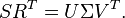
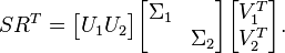
Next, the [[wikipedia:Singular_Value_Decomposition|Singular Value Decomposition]] of <math> SR^T\;</math> is computed: |
Next, the [[wikipedia:Singular_Value_Decomposition|Singular Value Decomposition]] of <math> SR^T\;</math> is computed: |
||
| Line 46: | Line 50: | ||
<math>SR^T= \begin{bmatrix} U_1 U_2 \end{bmatrix} \begin{bmatrix} \Sigma_1 & \\ & \Sigma_2\end{bmatrix} \begin{bmatrix} V_1^T\\V_2^T\end{bmatrix}.</math> |
<math>SR^T= \begin{bmatrix} U_1 U_2 \end{bmatrix} \begin{bmatrix} \Sigma_1 & \\ & \Sigma_2\end{bmatrix} \begin{bmatrix} V_1^T\\V_2^T\end{bmatrix}.</math> |
||
| − | The truncation of discardable partitions <math>U_2,V^T_2,\Sigma_2</math> results in the reduced order model <math>(P^TAQ,P^TB,CQ,D)\;</math> where |
+ | The truncation of discardable partitions <math>U_2,V^T_2,\Sigma_2</math> results in the reduced order model <math>(P^TEQ,P^TAQ,P^TB,CQ,D)\;</math> where |
| − | <math> P |
+ | <math> P^T=\Sigma_1^{-\frac{1}{2}}V_1^T R E^{-1},</math> |
<math> Q= S^T U_1 \Sigma_1^{-\frac{1}{2}}.</math> |
<math> Q= S^T U_1 \Sigma_1^{-\frac{1}{2}}.</math> |
||
| − | <math> |
+ | Note that <math>P^TEQ=I_r</math> which makes <math> QP^T</math> an oblique projector and hence '''Balanced Trunctation''' a Petrov-Galerkin projection method. The reduced model is stable with Hankel Singular Values given by <math>\sigma_1,\dots,\sigma_r</math>, where r is the order of the reduced system. It is possible to choose <math>r</math> via the computable error bound<ref>D.F. Enns, "<span class="plainlinks">[http://dx.doi.org/10.1109/CDC.1984.272286 Model reduction with balanced realizations: An error bound and a frequency weighted generalization]</span>," The 23rd IEEE Conference on Decision and Control, vol.23, pp.127,132, Dec. 1984</ref>: |
<math> \|\Sigma-\hat{\Sigma}\|_2 \leq 2 \|u\|_2 \sum_{k=r+1}^n\sigma_k. </math> |
<math> \|\Sigma-\hat{\Sigma}\|_2 \leq 2 \|u\|_2 \sum_{k=r+1}^n\sigma_k. </math> |
||
Revision as of 12:06, 29 April 2013
Balanced Truncation is an important projection model reduction method which delivers high quality reduced models by making an extra effort in choosing the projection subspaces.
Derivation
We consider linear time-invariant systems, defined in generalized state-space form by
where nonsingularity of  and stability (
 stable) is assumed.
A stable minimal (controllable and observable) system  , realized by
  ,
is called balanced[1], if the systems Controllability Gramian and Observability Gramian, i.e. the solutions
,
is called balanced[1], if the systems Controllability Gramian and Observability Gramian, i.e. the solutions  and
and  of the (generalized) Lyapunov equations


satisfy  with
with  .
Since in general, the spectrum of
.
Since in general, the spectrum of  are the squared Hankel Singular Values for such a balanced system, they are given by:
  .
.
An arbitrary system can be transformed into a balanced system  via a state-space transformation:

This transformed system has balanced Gramians  and
and  which are equal and diagonal.
The balanced systems states are ordered (descendingly) by how controllable and observable they are, thus allowing a partion of the form:
which are equal and diagonal.
The balanced systems states are ordered (descendingly) by how controllable and observable they are, thus allowing a partion of the form:
 .
.
By truncating the discardable states, the truncated reduced system is then given by 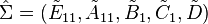 .
.
Implementation: SR Method
The necessary balancing transformation can be computed by the SR Method[2].
First, the Cholesky factors of the Gramians 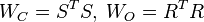 are computed.
Next, the Singular Value Decomposition of
are computed.
Next, the Singular Value Decomposition of  is computed:
Now, partitioning  , for example based on the Hankel singuar Values, gives
The truncation of discardable partitions  results in the reduced order model
  where
where
Note that  which makes
  an oblique projector and hence Balanced Trunctation a Petrov-Galerkin projection method. The reduced model is stable with Hankel Singular Values given by
  , where r is the order of the reduced system. It is possible to choose
  via the computable error bound[3]:
Direct Truncation
A related truncation-based approach is Direct Truncation[4].
Given a stable and symmetric system  , such that there exists a transformation


then the solution of the Sylvester Equation

is the Cross Gramian, of which the absolute value of its spectrum equals the Hankel Singular Values:
 .
.
Thus the Singular Value Decomposition of the Cross Gramian
also allows a partitioning
and a subsequent truncation of the discardable states, to which the above error bound also applies.
References
- ↑ B.C. Moore, "Principal component analysis in linear systems: Controllability, observability, and model reduction", IEEE Transactions on Automatic Control , vol.26, no.1, pp.17,32, Feb 1981
- ↑ A.J. Laub; M.T. Heath; C. Paige; R. Ward, "Computation of system balancing transformations and other applications of simultaneous diagonalization algorithms," IEEE Transactions on Automatic Control, vol.32, no.2, pp.115,122, Feb 1987
- ↑ D.F. Enns, "Model reduction with balanced realizations: An error bound and a frequency weighted generalization," The 23rd IEEE Conference on Decision and Control, vol.23, pp.127,132, Dec. 1984
- ↑ Antoulas, Athanasios C. "Approximation of large-scale dynamical systems". Vol. 6. Society for Industrial and Applied Mathematics, 2009; ISBN 978-0-89871-529-3