Moment-matching method

Description

The moment-matching methods are also called the Krylov subspace methods, as well as Padé approximation methods. They belongs to the Projection based MOR methods. These methods are applicable for non-parametric linear time invariant systems, often the descriptor systems, e.g.

$E \frac{dx(t)}{dt}=A x(t)+B u(t), \quad y(t)=Cx(t), \quad \quad (1)$

They are very efficient in many engineering applications, circuit simulation, Microelectromechanical systems (MEMS) simulation, etc..

The basic steps are as follows. First, the transfer function

$H(s)=Y(s)/U(s)=C(sE-A)^{-1}B$

is expanded into a power series at an expansion point $s_0\in\mathbb{C}\cup \infty$.

Let $s=s_0+\sigma$, then, within the convergence radius of the series, we have

$H(s_0 + \sigma)= C[(s_{0}+\sigma){E}-A]^{-1}B$

$=C[\sigma { E}+(s_{0}{ E}-{ A})]^{-1}B$

$=C[{ I}+\sigma(s_0{ E}-{ A})^{-1}E]^{-1}[(s_0{ E}-{ A})]^{-1}B$

$=C[{ I}-\sigma(s_0{ E}- A )^{-1}E+\sigma^2[(s_0{ E}-{ A})^{-1}E]^{2}+\ldots] s_0{E}-{ A})^{-1}B$

$=\sum \limits^\infty_{i=0}\underbrace{C[-(s_0{ E}-{A})^{-1}E]^i(s_0{ E}-{ A})^{-1}B}_{:= m_i(s_0)} \, \sigma^i,$

where $m_i(s_0)$ are called the moments of the transfer function about $s_0$ for $i=0,1,2,\ldots$. If the expansion point is chosen as zero then the moments simplify to $m_i(0)=C(A^{-1}E)^i(-A^{-1}B)$. For $s_0=\infty$ the moments are also called Markov parameters which can be computed by 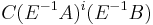$C(E^{-1}A)^i(E^{-1}B)$ if E is invertable.

The goal in moment-matching model reduction is the construction of a reduced order system where some moments $\hat m_i$ of the associated transfer function $\hat H$ match some moments of the original transfer function $H$.

The matrices $V$ and $W$ for model order reduction can be computed from the vectors which are associated with the moments, for example, using a single expansion point $s_0=0$, by

$\textrm{range}(V)=\textrm{span}\{\tilde B,({ A}^{-1}E)^2 \tilde B, \ldots,({ A}^{-1}E)^{r}{\tilde B}\},$

$\textrm{range}(W)=\textrm{span}\{C^T, E^T{ A}^{-T}C^T,(E^T{A}^{-T})^2C^T, \ldots ,(E^T{A}^{-T})^{r-1}C^T\},$

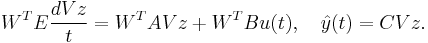
where $\tilde B=-A^{-1}B$. The reduced model is in the form as below

$W^TE \frac{d{V z}}{t}=W^TA Vz +W^T B u(t), \quad \hat{y}(t)=CVz.$

The transfer function $\hat H$ of the reduced model has good approximation properties around $s_0$, which matches the first $2r$ moments of $H(s)$ at $s_0$.

Using a set of $k$ distinct expansion points $\{s_1,\cdots,s_k\}$, the reduced model can be obtained by, e.g.,

$\textrm{range}(V)=\textrm{span}\{(A-s_1 {E})^{-1}E\tilde B,\ldots,(A-s_k {E})^{-1}E\tilde B \}$,

$\textrm{range}(W)=\textrm{span}\{E^T(A-s_1 {E})^{-T}C^T,\ldots,E^T(A-s_k {E})^{-T}C^T \},$

has order $r=k$ and matches the first two moments at each $s_j$, $j=1,\ldots,k$, see .

It can be seen that the columns of $V$, $W$ span Krylov subspaces which can easily be computed by Arnoldi or Lanczos methods . In these algorithms only matrix-vector multiplications are used which are simple to implement and the complexity of the resulting methods is only $O(n r^2)$.

References

- ↑ 1.0 1.1 R.W. Freund, "Model reduction methods based on Krylov subspaces". Acta Numerica, 12:267-319, 2003.
- ↑ 2.0 2.1 P. Feldmann and R.W. Freund, "Efficient linear circuit analysis by Pade approximation via the Lanczos process". IEEE Trans. Comput.-Aided Des. Integr. Circuits Syst., 14:639-649, 1995.
- ↑ Cite error: Invalid
<ref>tag; no text was provided for refs namedgrimme97