Synthetic parametric model

Introduction

On this page you will find a purely synthetic parametric model. The goal is to have a simple parametric model which one can use to experiment with different system orders, parameter values etc.

System description

The parameter $\varepsilon$ scales the real part of the system poles, that is, $p_i=\varepsilon a_i+jb_i$. For a system in pole-residue form

$H(s) = \sum_{i=1}^{n}\frac{r_i}{s-p_i} = \sum_{i=1}^{n}\frac{r_i}{s-(\varepsilon a_i+jb_i)} ,$

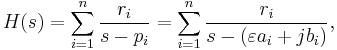
we can then write down the state-space realisation

$\widehat{A} = \varepsilon \left[\begin{array}{ccc} a_1 & & \\ & \ddots & \\ & & a_n\end{array}\right] +\left[\begin{array}{ccc} jb_1 & & \\ & \ddots & \\ & & jb_n\end{array}\right] = \varepsilon \widehat{A}_\varepsilon + \widehat{A}_0,$

$\widehat{B} = [1,\ldots,1]^T,\quad \widehat{C} = [r_1,\ldots,r_n],\quad D = 0.$

Notice that the system matrices have complex entries.

For simplicity, assume that $n$ is even, $n=2k$, and that all system poles are complex and ordered in complex conjugate pairs, i.e.

$p_1 = \varepsilon a_1+jb_1, p_2 = \varepsilon a_1-jb_1, \ldots, p_{n-1} = \varepsilon a_k+jb_k, p_n = \varepsilon a_k-jb_k,$

which also implies that the residues form complex conjugate pairs $r_1, \bar{r}_1,\ldots , r_k, \bar{r}_k.$

Then a realization with matrices having real entries is given by

$A = T\widehat{A}T^*, \quad B = T\widehat{B}, \quad C = \widehat{C}T^*, \quad D = 0,$

with $T = \left[\begin{array}{ccc} T_0 & & \\ & \ddots & \\ & & T_0 \end{array}\right]$, for $T_0 = \frac{1}{\sqrt{2}}\left[\begin{array}{cc} 1 & -j\\ 1 & j \end{array}\right]$.

Numerical values

The numerical values for the different variables are the following:

• the residues $r_i, i = 1,\ldots,k$ are real and equally spaced in $[10^{-3},1]$, with $r_1 = 1]$ and $r_k = 10^{-3}$.

• $\mathrm a_i, i = 1,\ldots,k$ linearly spaced between $[10^{-1},10^3]$,

• $\mathrm b_i, i = 1,\ldots,k$ linearly spaced between $[10,10^3]$,

• $\varepsilon \in [1,20]$,