Tunable Optical Filter

Tunable Optical Filter

Background
Benchmark ID	tunableOpticalFilter_n106437m1q5 tunableOpticalFilter_n1668m1q5
Category	oberwolfach
System-Class	LTI-FOS
Parameters
nstates	106437 1668
ninputs	1
noutputs	5
nparameters	0
components	A, B, C, E
Copyright
License	NA
Creator	Christian Himpe
Editor	Christian Himpe Steffen Werner
Location
NA

Description

Figure 1: Tunable optical filter.

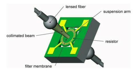
A benchmark for the heat transfer problem, related to modeling of a tunable optical filter (see Fig. 1), is presented. It can be used to apply model reduction algorithms to a linear first-order problem.

Modeling

The DFG project AFON (funded under grant ZA 276/2-1) aimed at the development of an optical filter, which is tunable by thermal means. The thin-film filter is configured as a membrane in order to improve thermal isolation. Fabrication is based on silicon technology. Wavelength tuning is achieved through thermal modulation of resonator optical thickness, using metal resistor deposited onto the membrane. The devices features low power consumption, high tuning speed and excellent optical performance. These tunable devices are an important component in various optical systems such as tunable lasers.

The benchmark contains a simplified thermal model of a filter device. It helps designers to consider important thermal issues, such as what electrical power should be applied in order to reach the critical temperature at the membrane or homogeneous temperature distribution over the membrane. The original model is the heat transfer partial differential equation

$\begin{align} \nabla \cdot (\kappa(r) \nabla T(r,t)) + Q(r, t) - \rho(r)C_{p}(r)\frac{\partial T(r, t)}{\partial t} & = 0, \end{align}$

where $r$ is the position, $t$ is the time, $\kappa$ is the thermal conductivity of the material, $C_{p}$ is the specific heat capacity, $\rho$ is the mass density, $Q$ is the heat generation rate that is nonzero only within the heater, and $T$ is the unknown temperature distribution to be determined.

There are two different benchmarks, 2D model and 3D model (see Table 1). Due to modeling differences, their simulation results cannot be compared with each other directly.

Table 1: Tunable optical filter benchmarks.

Code	Comment	Dimension	nnz(A)	nnz(E)
filter2D	2D, linear elements, PLANE55	1668	6209	1668
filter3D	3D, linear elements, SOLID90	108373	1406808	1406791

Discretization

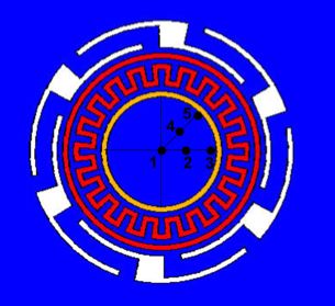
The solid device models have been designed, meshed and discretized in ANSYS 6.1 by the finite element method. All material properties are considered as temperature independent. Temperature is assumed to be in Celsius with the initial state of $0^{\circ}C$. The Dirichlet boundary conditions of $T = 0^{\circ}C$ have been applied at the bottom of the chip. Output nodes for the models are described in Table 2 and schematically displayed in Fig. 2. The first output is located at the very center of the membrane. By simulating its temperature one can prove how much input power is needed to reach the critical membrane temperature for each wavelength. Furthermore, the outputs 2 to 5 must be very close to output 1 (homogeneous temperature distribution) in order to provide the same optical properties across the complete diameter of the laser beam.

Table 2: Outputs for the optical filter model.

Number	Code	Comment
1	Memb1	Membrane center
2	Memb2	Membrane node with radius 25E-6, theta 90°
3	Memb3	Membrane node with radius 50E-6 theta 90°
4	Memb4	Membrane node with radius 25E-6, theta 135°
5	Memb5	Membrane node with radius 50E-6 theta 135°

Figure 2: Schematic position of the chosen output nodes.

The input corresponds to the constant power of of $1 mW$ for 2D model and $10 mW$ for 3D model. Hence practically, the benchmark contains a constant load vector. The linear ordinary differential equations of the first order are written as:

$\begin{align} E\dot{x}(t) &= Ax(t) + b,\\ y(t) &= Cx(t), \end{align}$

where $E$ and $A$ are the symmetric sparse system matrices (heat capacity and heat conductivity matrix), $b$ is the load vector, $C$ is the output matrix, and $x$ is the vector of unknown temperatures.

The output of the transient simulation for node 1 over the rise time of the device ($0.25 s$) for 3D model can be found in Filter3DTransResults. The results can be used to compare the solution of a reduced model with the original one. The time integration has been performed in ANSYS with accuracy of about $0.1\%$. The results are given as matrices where the first row is made of times, the second of the temperatures.

The discussion of electro-thermal modeling related to the benchmark can be found in.

Acknowledgments

This work is partially funded by the DFG projects AFON (ZA 276/2-1), MST-Compact (KO-1883/6) and an operating grant of the University of Freiburg.

Origin

This benchmark is part of the Oberwolfach Benchmark Collection; No. 38875, see: .

Data

This benchmark includes two data sets, one for the 2D and one for 3D model. The matrices can be downloaded in the Matrix Market format:

• TunableOpticalFilter-dim1e3-filter2D.tar.gz (104.0 kB)
• TunableOpticalFilter-dim1e5-filter3D.tar.gz (35.7 MB)

The matrix name is used as an extension of the matrix file. The file *.C.names contains a list of ouput names written consecutively. The file Filter3DTransResults contains the output of the transient simulation for node 1 over the rise time of the device ($0.25 s$) for the 3D model and Filter3DTransResults.names the corresponding output names. The system matrices have been extracted from ANSYS models by means of mor4fem.

Dimensions

System structure:

$\begin{align} E\dot{x}(t) &= Ax(t) + b,\\ y(t) &= Cx(t) \end{align}$

System dimensions:

$E \in \mathbb{R}^{N \times N}$, $A \in \mathbb{R}^{N \times N}$, $b \in \mathbb{R}^{N \times 1}$, $C \in \mathbb{R}^{5 \times N}$,

System variants:

filter2d: $N = 1668$, filter3d: $N = 108373$

Citation

To cite this benchmark, use the following references:

• For the benchmark itself and its data:

Oberwolfach Benchmark Collection, Tunable Optical Filter. hosted at MORwiki - Model Order Reduction Wiki, 2018. http://modelreduction.org/index.php/Tunable_Optical_Filter

@MISC{morwiki_optical,
  author =       {{Oberwolfach Benchmark Collection}},
  title =        {Tunable Optical Filter},
  howpublished = {hosted at {MORwiki} -- Model Order Reduction Wiki},
  url =          {https://modelreduction.org/morwiki/Tunable_Optical_Filter},
  year =         20XX
}

• For the background on the benchmark:

@ARTICLE{HohZ04,
  author =       {D. Hohlfeld and H. Zappe},
  title =        {An all-dielectric tunable optical filter based on the thermo-optic effect},
  journal =      {Journal of Optics A: Pure and Applied Optics},
  volume =       {6},
  number =       {6},
  pages =        {504--511},
  year =         {2004},
  doi =          {10.1088/1464-4258/6/6/002}
}

References

- ↑ D. Hohlfeld, H. Zappe, All-dielectric tunable optical filter based on the thermo-optic effect, Journal of Optics A: Pure and Applied Optics, 6(6): 504--511, 2004.
- ↑ T. Bechthold, Model order reduction of electro-thermal MEMS, Albert-Ludwigs-Universität Freiburg, 2005.
- ↑ J.G. Korvink, E.B. Rudnyi, Oberwolfach Benchmark Collection, Dimension Reduction of Large-Scale Systems, Lecture Notes in Computational Science and Engineering, vol 45: 311--315, 2005.
- ↑ D. Hohlfeld, T. Bechtold, H. Zappe, Tunable Optical Filter, Dimension Reduction of Large-Scale Systems, Lecture Notes in Computational Science and Engineering, vol 45: 337--340, 2005.