Batch Chromatography

Description

Figure 1: Sketch of a batch chromatographic process for the separation of A and B.

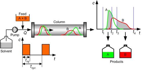
Preparative liquid chromatography as a crucial separation and purification tool has been widely employed in the food, fine chemical, and pharmaceutical industries. Chromatographic separation at the industry scale can be operated either discontinuously or in a continuous mode. The continuous case will be discussed in the benchmark SMB, and here we focus on the discontinuous mode -- batch chromatography. The principle of the batch chromatographic process for the binary separation is shown in Fig. 1. During the injection period \(t_{inj}\), a mixture of products A and B is injected at the inlet of the column packed with a suitable stationary phase. With the help of the mobile phase, the feed mixture flows through the column. Since the to-be-separated solutes exhibit different adsorption affinities to the stationary phase, they move at different velocities and thus separate from each other when exiting the column. At the column outlet, component A is collected between \(t_1\) and \(t_2\), and component B is collected between \(t_3\) and \(t_4\). Here the positions of \(t_1\) and \(t_4\) are determined by a minimum concentration threshold that the detector can resolve, and the positions of \(t_2\) and \(t_3\) are determined by the purity specifications imposed on the products. After the cycle period \(t_{cyc}:=t_4-t_1\), the injection is repeated. The feed flow rate \(Q\) and injection period \(t_{inj}\) are often considered as the operating variables. By properly choosing them, the process can achieve the desired performance criterion, such as production rate, while respecting the product specifications (e.g., purity, recovery yield).

The dynamics of the batch chromatographic column can be described precisely by an axially dispersed plug-flow model with a limited mass-transfer rate characterized by a linear driving force (LDF) approximation. In this model the differential mass balance of component \(i\) (\(i=A,B,\)) in the liquid phase can be written as:

\[ \frac{\partial c_i}{\partial t} + \frac{1 - \epsilon}{\epsilon} \frac{\partial q_i}{\partial t} + u \frac{\partial c_i}{\partial z} - D_i \frac{\partial^2 c_i}{\partial z^2} = 0, \qquad z \in (0, L), \qquad (1) \]

where \(c_i\) and \(q_i\) are the concentrations of solute \(i\) in the liquid and solid phases, respectively, \(u\) the interstitial liquid velocity, \(\epsilon\) the column porosity, \(t\) the time coordinate, \(z\) the axial coordinate along the column, \(L\) the column length, \(D_i=\frac{uL}{Pe}\) the axial dispersion coefficient and \(Pe\) the Péclet number. The adsorption rate is modeled by the LDF approximation:

\[ \frac{\partial q_i}{\partial t} = \kappa_{i} \left(q^{Eq}_i - q_i\right), \qquad z \in [0, L], \]

where \(\kappa_{i}\) is the mass-transfer coefficient of component \(i\) and \(q^{Eq}_i\) is the adsorption equilibrium concentration calculated by the isotherm equation for component \(i\). Here the bi-Langmuir isotherm model is used to describe the adsorption equilibrium:

\[ q^{Eq}_i = \frac{H_{i,1}\,c_i}{1 + \sum_{j = A, B}K_{j,1}\,c_j} + \frac{H_{i,2}\,c_i}{1 + \sum_{j = A, B}K_{j,2}\,c_j},\; i = A, B, \]

where \(H_{i,1}\) and \(H_{i,2}\) are the Henry constants, and \(K_{j,1}\) and \(K_{j,2}\) the thermodynamic coefficients.

The boundary conditions for (1) are specified by the Danckwerts relations:

\[ D_i \left.\frac{\partial c_i}{\partial z}\right|_{z = 0} = u \left(\left.c_i\right|_{z=0} - c^{in}_i\right), \qquad \left.\frac{\partial c_i}{\partial z}\right|_{z = L} = 0, \]

where \(c^{in}_i\) is the concentration of component \(i\) at the inlet of the column. A rectangular injection is assumed for the system and thus

\[ c^{in}_i = \begin{cases} c^F_i, & \text{if } t \le t_{inj}, \\ 0, & \text{if } t > t_{inj}. \end{cases} \]

Here \(c^F_i\) is the feed concentration for component \(i\) and \(t_{inj}\) is the injection period. In addition, the column is assumed unloaded initially:

\[ c_i(t = 0, z) = q_i(t = 0,z) = 0, \quad z \in [0, L], \; i = A, B. \]

More details about the mathematical modeling for batch chromatography can be found in the literature .

Discretization

In this model, the feed volumetric flow-rate \(Q\) and the injection period \(t_{inj}\) are considered as the operating parameters, and denoted as the parameter \(\mu=(Q,\,t_{inj})\). Using the finite volume discretization, we get the full order model (FOM) as follows,

\[ \left\{ \begin{aligned} \mathbf{A} \mathbf{c}_i^{k+1} &= \mathbf{B} \mathbf{c}_i^{k} + d_i^k - \frac{1 - \epsilon}{\epsilon} \Delta t \mathbf{h}_i^k, \\ \mathbf{q}_i^{k + 1} &= \mathbf{q}_i^{k} + \Delta t \mathbf{h}_i^k, \end{aligned} \right. \]

where \(\mathbf{c}_i^k, \mathbf{q}_i^k \in \mathbb{R}^{\mathcal N}, i = A, B\) are the solution vectors of \(c_i\) and \(q_i\) at the time instance \(t = t^k, k = 0, 1, \ldots, K\), respectively. The time step \(\Delta t \) is determined by the stability condition. The equation \( \mathbf h_i^k = \kappa_{i} (\mathbf q^{Eq}_i - \mathbf q_i^k) \), is time- and parameter-dependent, the boldface \(\mathbf{A,B}\) are constant matrices. As a result, it is a nonlinear parametric system.

Generation of ROM

The reduced order model (ROM) can be obtained by the reduced basis method , which is applicable for nonlinear parametric systems, see Reduced Basis PMOR method. For parametrized time-dependent problems, the reduced basis is often generated by using the POD-Greedy algorithm . Notice that the nonlinear functions \(\mathbf h_i, i=A, B\) can be approximated by the empirical interpolation method , such that the ROM can be obtained efficiently by the strategy of offline-online decomposition.

Assume \(W_z\) is the collateral reduced basis (CRB) for the nonlinear operator \(h_z\), and \(V_{c_z},V_{q_z}\) are the reduced bases for the field variables \(c_z\) and \(q_z\), respectively. Applying Galerkin projection and empirical operator interpolation, the ROM can be formulated as:

\[ \left\{ \begin{aligned} \hat{A}_{c_z} {a}_{c_z}^{n+1} &= \hat{B}_{c_z} {a}_{c_z}^{n} + d_0^n \hat{d}_{c_z} - \frac{1 - \epsilon}{\epsilon} \Delta t \hat{H}_{c_z} \beta_z^n, \\ {a}_{q_z}^{n + 1} &= {a}_{q_z}^{n} + \Delta t \hat{H}_{q_z} \beta_z^n, \end{aligned} \right. \]

where \( {a}_{c_z}^n, {a}_{q_z}^n \in \mathbb R^N\) are the solution of the ROM. \(\hat{A}_{c_z}=V_{c_z}^T A V_{c_z}, \hat{ B}_{c_z}=V_{c_z}^T B V_{c_z}, \hat{d}_{c_z}^{n}=V_{c_z}^T e_1\), \(\hat{H}_{c_z}:= V_{c_z}^TW_z ,\) \(\hat{H}_{q_z}:= V_{q_z}^TW_z \) are the reduced matrices, \(e_1:=(1,0,\cdots,0)\). \(\beta_z^n \in \mathbb R^M\) is the coefficients of the CRB \(W_z\) for the empirical interpolation.

Data

Figure 2: Concentrations at the outlet of the column.

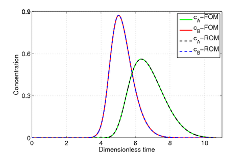
Fig. 2 shows the concentrations at the outlet of the column at a given parameter \(\mu= (0.1018, 1.3487)\), which show that the ROM (\(N=46, M=151\)) reproduces the dynamics of the full order model (\(\mathcal N=1000\)).

Citation

To cite this benchmark, use the following references:

• For the benchmark itself and its data:

The MORwiki Community, Batch Chromatography. MORwiki - Model Order Reduction Wiki, 2018. http://modelreduction.org/index.php/Batch_Chromatography

@MISC{morwiki_bone,
  author =       {{The MORwiki Community}},
  title =        {Batch Chromatography},
  howpublished = {{MORwiki} -- Model Order Reduction Wiki},
  url =          {https://modelreduction.org/morwiki/index.php/Batch_Chromatography},
  year =         {2018}
}

• For the background on the benchmark:

@ARTICLE{RieWHetal95,
  author =       {Y. Zhang and L. Feng and S. Li and P. Benner},
  title =        {Accelerating {PDE} constrained optimization by the reduced basis method: application to batch chromatography},
  journal =      {International Journal for Numerical Methods in Engineering},
  volume =       {104},
  number =       {11},
  pages =        {983--1007},
  year =         {2015},
  doi =          {10.1002/nme.4950}
}

Contact

Yongjin Zhang

Suzhou Li

References

- ↑ G. Guiochon, A. Felinger, D. G. Shirazi, A. M. Katti, Fundamentals of Preparative and Nonlinear Chromatography, 2nd Edition, Academic Press, 2006.
- ↑ Y. Zhang, L. Feng, S. Li and P. Benner, "Accelerating PDE constrained optimization by the reduced basis method: application to batch chromatography", International Journal for Numerical Methods in Engineering, 104(11): 983--1007, 2015.
- ↑ B. Haasdonk and M. Ohlberger, "Reduced basis method for finite volume approximations of parameterized linear evolution equations", Mathematical Modeling and Numerical Analysis, 42 (2008), 277-302.
- ↑ M. Barrault, Y. Maday, N.C. Nguyen, and A.T. Patera, "An 'empirical interpolation' method: application to efficient reduced-basis discretization of partial differential equations", C. R. Acad. Sci. Paris Series I, 339 (2004), 667-672.